Example notebook for implementing numerical propagation using propagate module
In the following we exemplify Rayleigh-Sommerfeld (RS), Bluestein, Angular Spectrum Method (ASM) and Scalable Angular Spectrum Method (SASM) propagations available in pyMOE using the propagate module. In particular:
Several examples of RS propagations in Z axis, YZ and XY planes:
RS, ASM and Bluestein propagation from elements defined from library functions apertures (e.g. Fresnel lenses)
RS, ASM and Bluestein propagation from elements defined from arbitrarily defined functions (e.g. Spiral Phase Plate)
Some examples comprise comparison of propagation results among RS, Bluestein, ASM and and SASM
In the propagate module, RS propagation is implemented via direct numerical integration of a double integral (see, e.g. Goodman Fourier Optics textbook as reference), making it (very) time-consuming, yet exact. The Bluestein method was implemented as https://www.nature.com/articles/s41377-020-00362-z - for this method, validity ranges are same as Fresnel propagation, hence please use with caution. The SASM is implemented following
https://opg.optica.org/optica/fulltext.cfm?uri=optica-10-11-1407.
Fresnel and Fraunhofer propagations provide acceptable approximations with faster computation for the propagation in some ranges. In the propagate module these approximations have been implemented following the Goodman Fourier Optics textbook. For simple use examples of Fresnel and Fraunhofer propagations check propopt package https://github.com/cunhaJ/propopt .
[1]:
# Notebook display options, change as your preference/system
%matplotlib inline
%config InlineBackend.print_figure_kwargs={'facecolor' : "w",'bbox_inches':None}

import matplotlib as mpl
mpl.rcParams['figure.dpi'] = 120
[2]:
# auto reload
%load_ext autoreload
%autoreload 2
[3]:
import sys
sys.path.insert(0,'..')
sys.path.insert(0,'../..')

from matplotlib import pyplot as plt
import numpy as np

from scipy.constants import micro, nano, milli

import pyMOE as moe
# from pyMOE.generate import *
# from pyMOE.propagate import *
Propagation from a circular aperture
[4]:
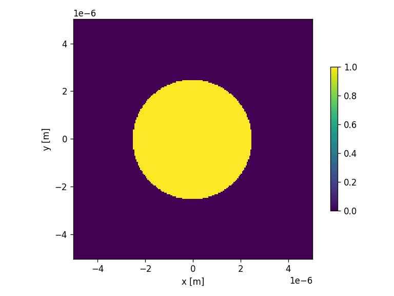
# Make circular apertures (returns also the 2D array)
wavelength = 400e-9 #m
zdist = 100*wavelength #m
pixsize = 0.1 * wavelength
x_pixel = 100
y_pixel = 100
aperture_width = x_pixel*pixsize
aperture_height = y_pixel*pixsize
radius = 1000e-9 #m
# Define Aperture
aperture = moe.generate.create_empty_aperture(-aperture_width/2, aperture_width/2, x_pixel, -aperture_height/2, aperture_height/2, y_pixel)
# Populate Aperture from phase mask
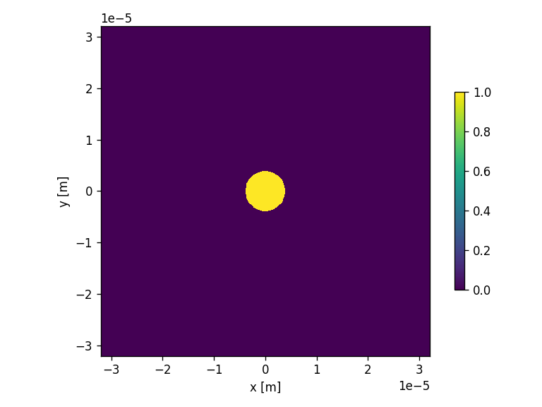
mask = moe.generate.circular_aperture(aperture, radius=radius)
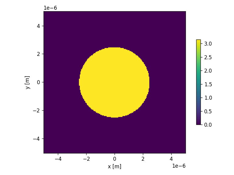
# Define Phase mask
mask_phase = moe.generate.create_empty_aperture_from_aperture(aperture)
mask_phase.aperture = mask.aperture*np.pi
# Plot the circular mask
moe.plotting.plot_aperture(mask)

[5]:
# Calculates a field to use with the calculated mask
# Initialize a Field from the Aperture mask
field = moe.field.create_empty_field_from_aperture(mask)
# Generate a uniform field
field = moe.field.generate_uniform_field(field, E0=1)
# Or Gaussian field is also available
#field = moe.field.generate_gaussian_field(field, E0=1, w0=100*micro)
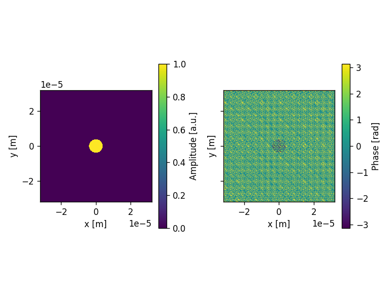
# Modulates the field with a given aperture that can be used either as an amplitude mask or a phase mask
field = moe.field.modulate_field(field, amplitude_mask=mask, phase_mask=None)
# Plots the field (amplitude and phase)
moe.plotting.plot_field(field)
plt.tight_layout()
plt.show()
[6]:
####Propagate field and calculate in plane YZ, using npix bins in Y
#Using RS propagation, the most exact
zmin = wavelength
zmax = 0.2*zdist
nzs = 50

# Creates a screen in YZ plane with [-aperture_height/2, aperture_height/2] and [zmin, zmax] and
screen_YZ = moe.field.create_screen_YZ(-aperture_height/2, aperture_height/2, y_pixel,
                                        zmin, zmax, nzs,
                                        x=0)

# Propagate the field
E_YZ = moe.propagate.RS_integral(field, screen_YZ, wavelength, simp2d=True)
[########################################] | 100% Completed | 11.57 s
[7]:
x = np.linspace(0,10, 10,)
y = np.linspace(0,20, 20)
z = np.linspace(0,30, 30)
X, Y, Z = np.meshgrid(x,y,z, indexing='ij')


Z.shape
[7]:
(10, 20, 30)
[8]:
#Plot the amplitude of the propagated field in yz screen
moe.plotting.plot_screen_YZ(E_YZ, which='amplitude')
plt.show()

#Plot the phase of the propagated field in yz screen
moe.plotting.plot_screen_YZ(E_YZ, which='phase')
plt.show()
[9]:
###Plot intensity in the YZ screen
I_YZ= E_YZ
I_YZ.screen= np.abs(E_YZ.amplitude)**2 ## careful with multiple assertions this way

moe.plotting.plot_screen_YZ(I_YZ, which='amplitude', colorbar=False)
plt.colorbar(label='Intensity [a.u.]')
plt.title("Intensity")
plt.show()
[10]:
###Propagate field using Bluestein
zmin = wavelength*2
zmax = 0.1*zdist*1
nzs = 200
# Creates a screen in YZ plane with [-aperture_height/2, aperture_height/2] and [zmin, zmax] and
ymin, ymax = -aperture_height/2, aperture_height/2
xmin, xmax = -aperture_height/2, aperture_height/2
x = np.linspace(xmin, xmax, x_pixel)
y = np.linspace(ymin, ymax, y_pixel)
z = np.linspace(zmin, zmax, nzs)
screen = moe.Screen(x,y,z)
# Propagate the field
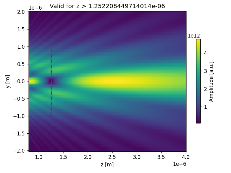
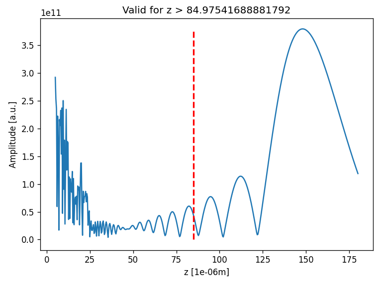
EXYZ_BS = moe.propagate.Bluestein(field, screen, wavelength)
print("Eyz shape:", EXYZ_BS.screen.shape)
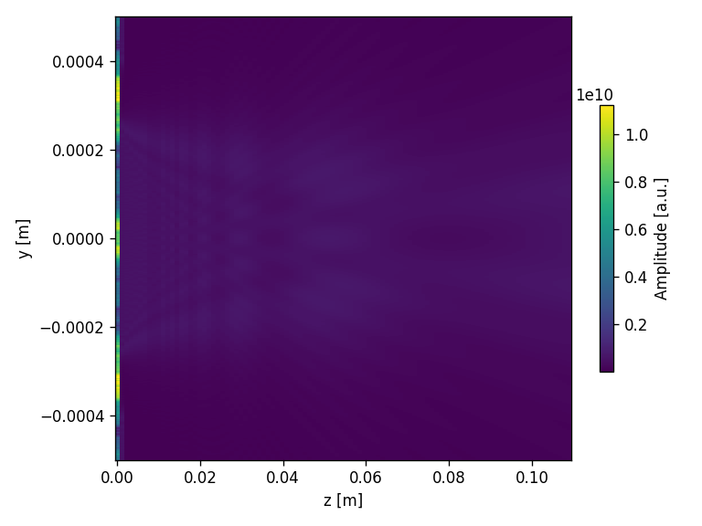
moe.plotting.plot_screen_YZ(EXYZ_BS, x=0, which='amplitude')
limitx = moe.propagate.Fresnel_criterion(wavelength,radius)
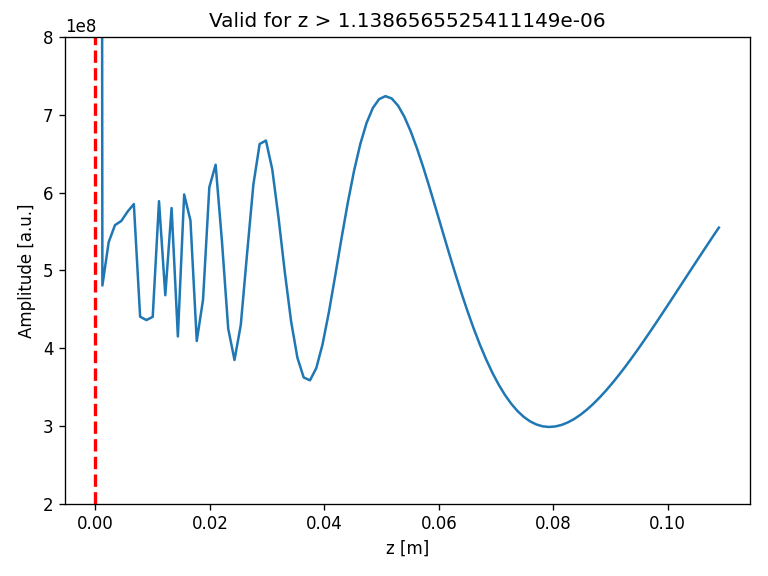
plt.vlines(limitx, -radius, radius, colors='red', linestyles='dashed', lw=2)
plt.title("Valid for z > "+str(limitx))
plt.show()
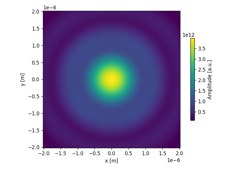
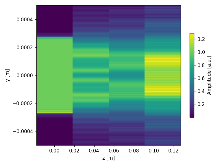
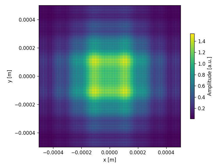
moe.plotting.plot_screen_XY(EXYZ_BS, z=zmax, which='amplitude')
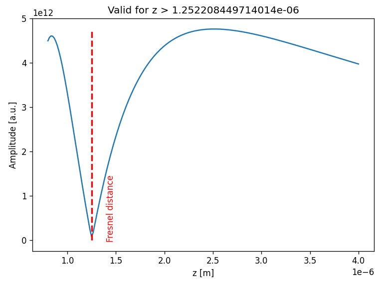
moe.plotting.plot_screen_ZZ(EXYZ_BS, which='amplitude')
limitx = moe.propagate.Fresnel_criterion(wavelength,radius)
plt.vlines(limitx, 0, np.max(EXYZ_BS.screen), colors='red', linestyles='dashed', lw=2)
plt.title("Valid for z > "+str(limitx))
plt.annotate("Fresnel distance", (1.4e-6,0.5e-6), rotation="vertical", color="Red")
plt.show()
Progress: [####################] 100.0%
Elapsed: 0:00:00.939949
Eyz shape: (100, 100, 200)
C:\ProgramData\anaconda3\Lib\site-packages\numpy\ma\core.py:3375: ComplexWarning: Casting complex values to real discards the imaginary part
  _data[indx] = dval
Propagate field using Angular Spectrum Method
[11]:
### Propagate field using Angular Spectrum Method
zmin = wavelength*2
zmax = 0.1*zdist*1
nzs = 200
# Creates a screen in YZ plane with [-aperture_height/2, aperture_height/2] and [zmin, zmax] and
ymin, ymax = -aperture_height/2, aperture_height/2
xmin, xmax = -aperture_height/2, aperture_height/2
x = np.linspace(xmin, xmax, x_pixel)
y = np.linspace(ymin, ymax, y_pixel)
z = np.linspace(zmin, zmax, nzs)
screen = moe.Screen(x,y,z)
# Propagate the field
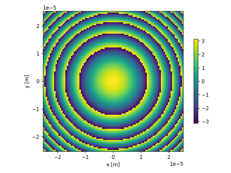
EXYZ_ASM = moe.propagate.ASM(field, screen, wavelength, pad=200)
# Eyz = EXYZ
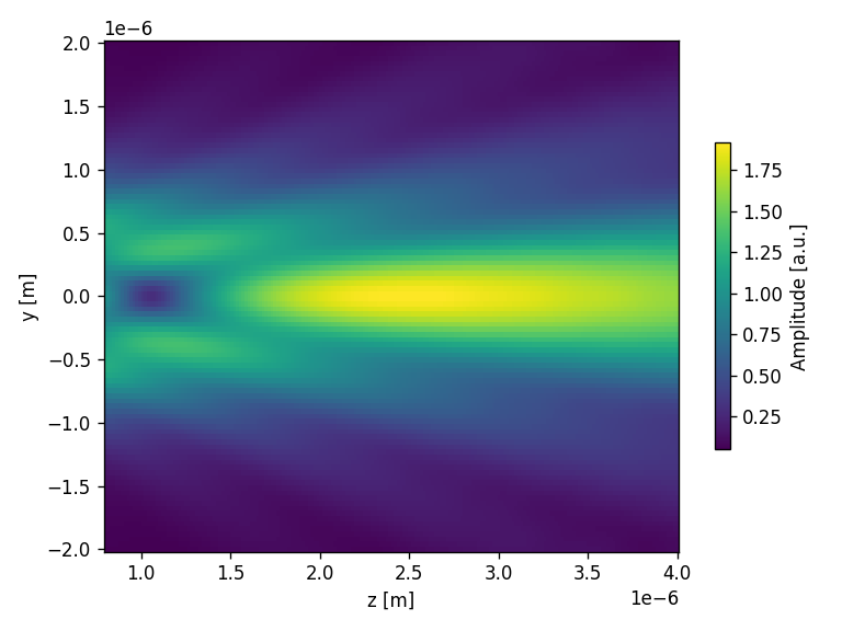
moe.plotting.plot_screen_YZ(EXYZ_ASM, which='amplitude')
plt.show()
moe.plotting.plot_screen_XY(EXYZ_ASM, which='amplitude')
moe.plotting.plot_screen_ZZ(EXYZ_ASM, which='amplitude')
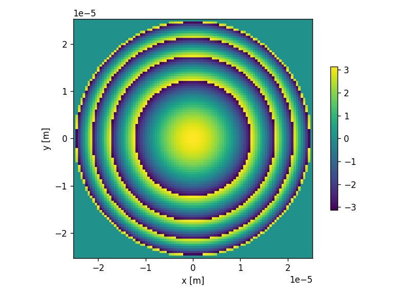
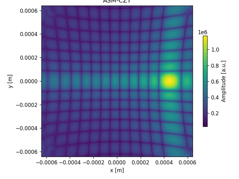
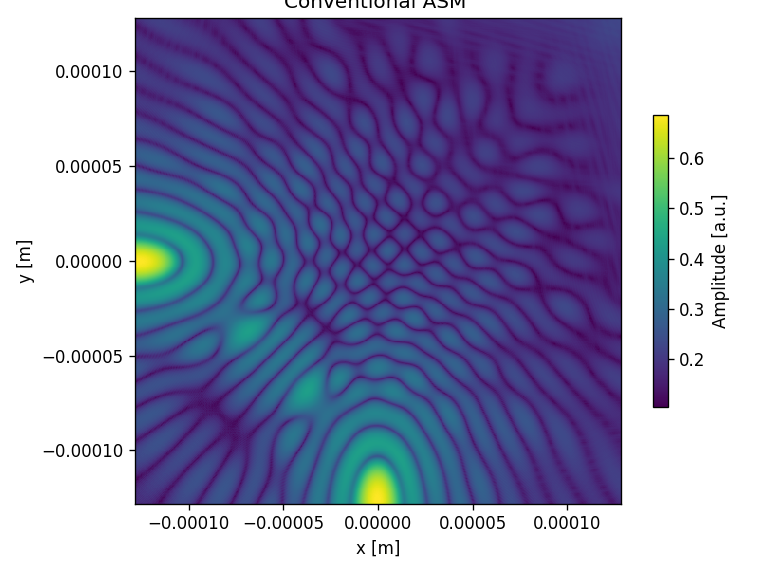
EXYZ_ASM = moe.propagate.ASM(field, screen, wavelength, pad=200, mode = "czt")
# Eyz = EXYZ
moe.plotting.plot_screen_YZ(EXYZ_ASM, which='amplitude')
plt.show()
moe.plotting.plot_screen_XY(EXYZ_ASM, which='amplitude')
moe.plotting.plot_screen_ZZ(EXYZ_ASM, which='amplitude')
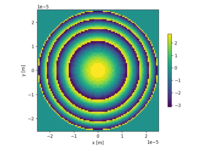
# Propagate the field
EXYZ_ASM = moe.propagate.ASM(field, screen, wavelength, pad=200, bl=True)
# Eyz = EXYZ
moe.plotting.plot_screen_YZ(EXYZ_ASM, which='amplitude')
plt.show()
moe.plotting.plot_screen_XY(EXYZ_ASM, which='amplitude')
moe.plotting.plot_screen_ZZ(EXYZ_ASM, which='amplitude')
Conventional ASM, without band limit.
C:\ProgramData\anaconda3\Lib\site-packages\paramiko\transport.py:219: CryptographyDeprecationWarning: Blowfish has been deprecated
  "class": algorithms.Blowfish,
Progress: [####################] 100.0%
Elapsed: 0:00:32.403723
ASM-CZT mode ON, without band limit.
Progress: [####################] 100.0%
Elapsed: 0:00:32.536606

Conventional ASM, with band limit.
Progress: [####################] 100.0%
Elapsed: 0:00:33.527930

[12]:
# Propagates the field in a single line along the Z axis
screen_ZZ = moe.field.create_screen_ZZ(zmin, zmax, nzs)
screen_ZZ = moe.propagate.RS_integral(field, screen_ZZ, wavelength, parallel_computing=True)

#moe.plotting.plot_screen_ZZ(screen_ZZ, which='amplitude')
[########################################] | 100% Completed | 661.21 ms
[13]:
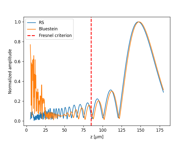
#Compare both propagations


normASM = np.abs(EXYZ_ASM.slice_Z(0,0))/np.max(np.abs(EXYZ_ASM.slice_Z(0,0)))
normBS  = np.abs(EXYZ_BS.slice_Z(0,0))/np.max(np.abs(EXYZ_BS.slice_Z(0,0)))
normRS  = np.abs(screen_ZZ.slice_Z(0,0))/np.max(np.abs(screen_ZZ.slice_Z(0,0)))


fig = plt.figure()

plt.plot(screen_ZZ.z, normRS, label="RS")

plt.plot(EXYZ_ASM.z, normASM, label ="ASM")
plt.plot(EXYZ_BS.z, normBS, label ="Bluestein")

plt.xlabel("z [m]")
plt.ylabel("Normalized amplitude")

plt.vlines(limitx, 0, 1, colors='red', linestyles='dashed', lw=2)
plt.legend()
#plt.annotate("Fresnel distance", (1.4e-6,0.5e-6), rotation="vertical", color="Red")
plt.title("Valid for z > "+str(limitx))
plt.annotate("Fresnel distance", (1.4e-6,0.5e-6), rotation="vertical", color="Red")
[13]:
Text(1.4e-06, 5e-07, 'Fresnel distance')
[14]:
fig = plt.figure()


phaseASM = np.angle(EXYZ_ASM.slice_Z(0,0))
phaseBS  = np.angle(EXYZ_BS.slice_Z(0,0))
phaseRS  = np.angle(screen_ZZ.slice_Z(0,0))


plt.plot(screen_ZZ.z, phaseRS, label="RS")
plt.plot(EXYZ_BS.z, phaseBS, label ="Bluestein")
plt.plot(EXYZ_ASM.z, phaseASM, label ="ASM")


plt.xlabel("z [m]")
plt.ylabel("Phase")

plt.vlines(limitx, -3.14, 3.14, colors='red', linestyles='dashed', lw=2)
plt.legend()
#plt.annotate("Fresnel distance", (1.4e-6,0.5e-6), rotation="vertical", color="Red")
plt.title("Valid for z > "+str(limitx))
plt.annotate("Fresnel distance", (1.3e-6,-3), rotation="vertical", color="Red")
[14]:
Text(1.3e-06, -3, 'Fresnel distance')

[15]:
# Propagate the field
EXYZ_CZT = moe.propagate.ASM(field, screen, wavelength, pad=200, bl=True, mode="czt")
ASM-CZT mode ON, with band limit.
Progress: [####################] 100.0%
Elapsed: 0:00:35.507584
[16]:
#Compare both propagations
normCZT = np.abs(EXYZ_CZT.slice_Z(0,0))/np.max(np.abs(EXYZ_ASM.slice_Z(0,0)))

phaseCZT = np.angle(EXYZ_CZT.slice_Z(0,0))


fig = plt.figure()

plt.plot(screen_ZZ.z, normRS, label="RS")
plt.plot(EXYZ_BS.z, normBS, label ="Bluestein")
plt.plot(EXYZ_ASM.z, normASM, label ="ASM", ls='--')
plt.plot(EXYZ_CZT.z, normCZT, label ="ASM CZT", ls='--')

plt.xlabel("z [m]")
plt.ylabel("Normalized amplitude")

plt.vlines(limitx, 0, 1, colors='red', linestyles='dashed', lw=2)
plt.legend()
#plt.annotate("Fresnel distance", (1.4e-6,0.5e-6), rotation="vertical", color="Red")
plt.title("Valid for z > "+str(limitx))
plt.annotate("Fresnel distance", (1.4e-6,0.5e-6), rotation="vertical", color="Red")

fig = plt.figure()


plt.plot(screen_ZZ.z, phaseRS, label="RS")
plt.plot(EXYZ_BS.z, phaseBS, label ="Bluestein")
plt.plot(EXYZ_ASM.z, phaseASM, label ="ASM", ls='--')
plt.plot(EXYZ_CZT.z, phaseCZT, label ="ASM CZT", ls='--')


plt.xlabel("z [m]")
plt.ylabel("Phase")

plt.vlines(limitx, -3.14, 3.14, colors='red', linestyles='dashed', lw=2)
plt.legend()
#plt.annotate("Fresnel distance", (1.4e-6,0.5e-6), rotation="vertical", color="Red")
plt.title("Valid for z > "+str(limitx))
plt.annotate("Fresnel distance", (1.1e-6,-3), rotation="vertical", color="Red")
[16]:
Text(1.1e-06, -3, 'Fresnel distance')
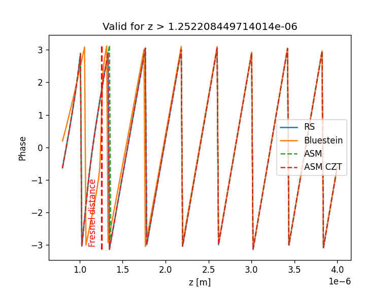
The ASM-CZT phase seems off in z, might miss either z related phase or unwrapping issue due to CZT freqs, use with care.
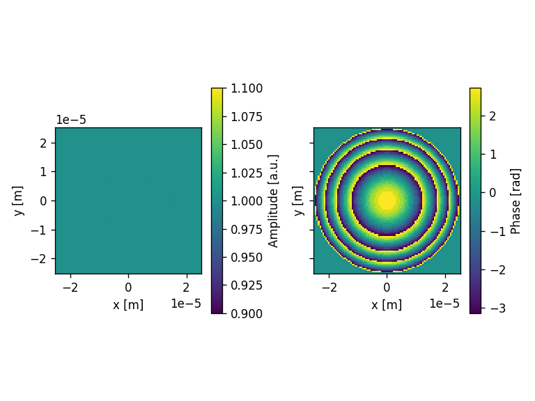
Propagation from a Fresnel multilevel mask example #1
Create the Fresnel aperture
[17]:
#number of pixels
x_pixel = 100
y_pixel = 100
#size of the rectangular mask
aperture_width = 50e-6 #m
aperture_height = 50e-6
pixsize = 1e-6 #m
wavelength = 500e-9 #m
focal_length = 150e-6
zmin = wavelength*20
zmax = 1.2* focal_length
nzs = 100
radius = aperture_width/2
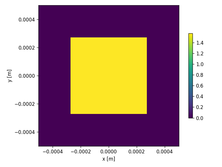
# Create Aperture
aperture1 = moe.generate.create_empty_aperture(-aperture_width/2, aperture_width/2, x_pixel, -aperture_height/2, aperture_height/2, y_pixel)
# Populate Aperture with Fresnel mask
mask1 = moe.generate.fresnel_phase(aperture1, focal_length, wavelength )
moe.plotting.plot_aperture(mask1)
##############
###Fresnel mask with a truncated circular aperture
# Create empty mask
aperture2 = moe.generate.create_empty_aperture_from_aperture(aperture1)
# and truncate around radius
mask2 = moe.generate.fresnel_phase(aperture2, focal_length, wavelength, radius=radius)
moe.plotting.plot_aperture(mask2)
# Discretize mask in number of levels
# Select exact position of contours in phase
phase_vals = np.linspace(-np.pi, np.pi, 16)
mask2.discretize(np.array( phase_vals)[:] )
moe.plotting.plot_aperture(mask2)
[18]:
### Create and modulate the uniform field
[19]:
# Generate a uniform field
field = moe.field.create_empty_field_from_aperture(mask2)

field = moe.field.generate_uniform_field(field, E0=1)

# Modulates the field
field = moe.field.modulate_field(field, amplitude_mask=None, phase_mask=mask2 )

# Plots the field (amplitude and phase)
moe.plotting.plot_field(field)

plt.tight_layout()
plt.show()
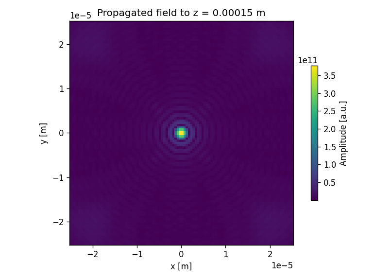
Propagate XY using Rayleigh-Sommerfeld and Bluestein
[20]:
##Propagate field in plane XY at z_distance

z_distance = focal_length

# Creates XY screen
screen_XY = moe.field.create_screen_XY(-aperture_width/2, aperture_width/2, x_pixel,
                                       -aperture_height/2, aperture_height/2, y_pixel,
                                        z=z_distance)

# Propagate the field
E_XY = moe.propagate.RS_integral(field, screen_XY, wavelength, simp2d=True)
E_XY_BS = moe.propagate.Bluestein(field, screen_XY, wavelength)
Warning: Sampling field pixel is larger than wavelength/2!
[########################################] | 100% Completed | 23.73 s
Progress: [####################] 100.0%
Elapsed: 0:00:00.006970
[21]:
# Plot the amplitude of the propagated field in XY screen

moe.plotting.plot_screen_XY(E_XY, which='amplitude')
plt.title("Propagated field to z = "+str(z_distance)+" m")

plt.tight_layout()
plt.show()
moe.plotting.plot_screen_XY(E_XY_BS, which='amplitude')
plt.title("Propagated field to z = "+str(z_distance)+" m")

plt.tight_layout()

plt.savefig("FresnelN16-XY.png")

plt.show()

Propagate YZ using Rayleigh-Sommerfeld
[22]:
#### Propagate field and calculate in plane YZ, using 100 bins in Y

nbins_y= 20

# Creates YZ screen
screen_YZ = moe.field.create_screen_YZ(-aperture_height/2, aperture_height/2, nbins_y,
                                        zmin, zmax, nzs,
                                        x=0)

# Propagate the field
E_YZ = moe.propagate.RS_integral(field, screen_YZ, wavelength, simp2d=True)
Warning: Sampling field pixel is larger than wavelength/2!
[########################################] | 100% Completed | 4.41 sms
[23]:
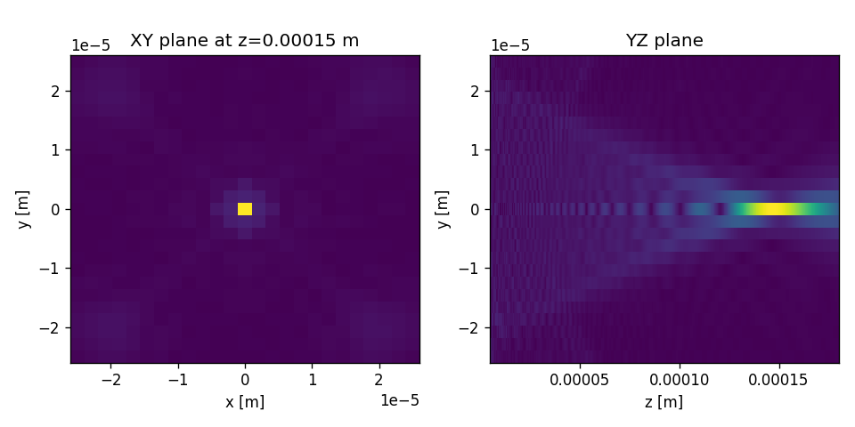
###Plot the two fields in same panel
fig = plt.figure(figsize=(8,4))
ax1 = fig.add_subplot(121)
ax2 = fig.add_subplot(122)


xp1 = E_XY.x
yp1 = E_XY.y
z1 = E_XY.slice_XY(z=focal_length)

yp2 = E_YZ.y
zp2 = E_YZ.z
z2 = E_YZ.slice_YZ(x=0)


ax1.title.set_text('XY plane at z='+str(focal_length)+' m')
ax1.pcolormesh(xp1,yp1,np.abs(z1) )
ax2.title.set_text('YZ plane')
ax2.pcolormesh(zp2,yp2,np.abs(z2) )


ax1.set(xlabel="x [m]", ylabel="y [m]")
ax2.set(xlabel="z [m]", ylabel="y [m]")

plt.tight_layout()

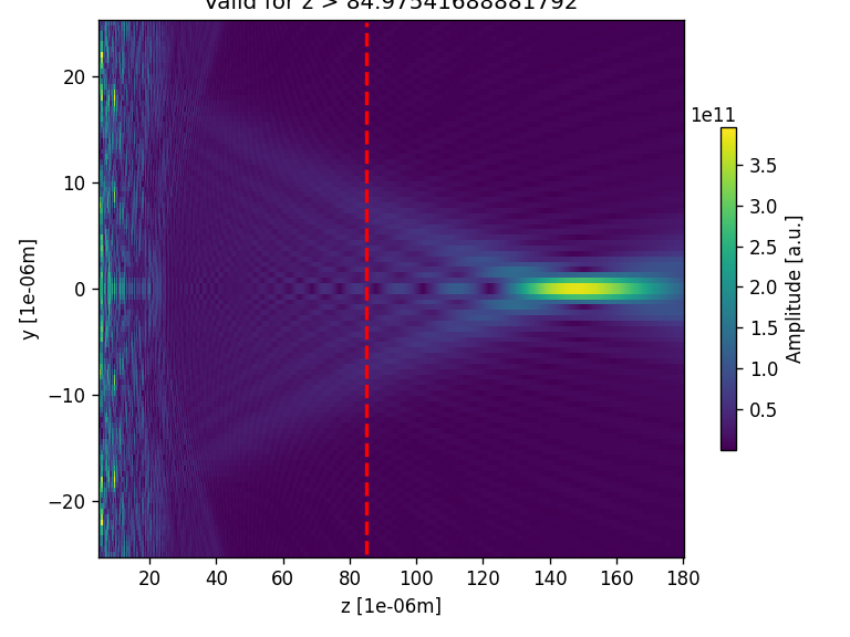
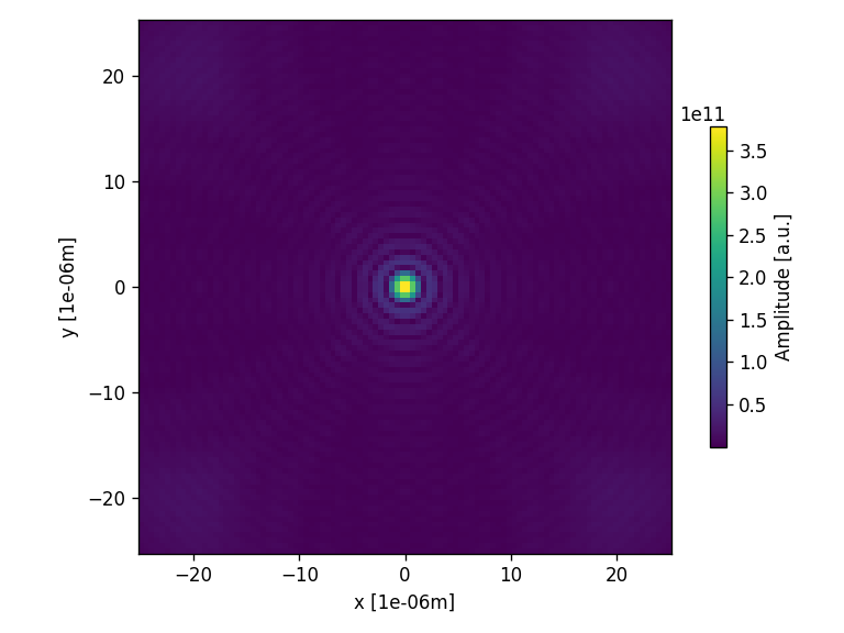
Propagate XYZ volume with Bluestein
[24]:
#Propagation using Bluestein

###Propagate field *10and calculate in plane YZ, using npix bins in Y
zmin = wavelength*10
zmax = 1.2* focal_length
nzs = 500

scale = 1e-6


# Creates a screen in YZ plane with [-aperture_height/2, aperture_height/2] and [zmin, zmax] and
ymin, ymax = -aperture_height/2, aperture_height/2
xmin, xmax = -aperture_width/2, aperture_width/2

x = np.linspace(xmin, xmax, x_pixel)
y = np.linspace(ymin, ymax, y_pixel)
z = np.linspace(zmin, zmax, nzs)


screen = moe.Screen(x,y,z)

# Propagate the field
EXYZ = moe.propagate.Bluestein(field, screen, wavelength)

moe.plotting.plot_screen_YZ(EXYZ, which='amplitude', scale=scale)

limitx = moe.propagate.Fresnel_criterion(wavelength,radius)/scale
plt.vlines(limitx, -radius/scale, radius/scale, colors='red', linestyles='dashed', lw=2)

plt.title("Valid for z > "+str(limitx))

plt.show()

moe.plotting.plot_screen_XY(EXYZ,z=focal_length, which='amplitude', scale=scale)

moe.plotting.plot_screen_ZZ(EXYZ,x=0,y=0, which='amplitude', scale=scale)

limitx = moe.propagate.Fresnel_criterion(wavelength,radius)/scale
plt.vlines(limitx, 0, np.max(EXYZ.screen), colors='red', linestyles='dashed', lw=2)

plt.title("Valid for z > "+str(limitx))

plt.show()
Progress: [####################] 100.0%
Elapsed: 0:00:02.448620
C:\ProgramData\anaconda3\Lib\site-packages\numpy\ma\core.py:3375: ComplexWarning: Casting complex values to real discards the imaginary part
  _data[indx] = dval
Compare ZZ between RS and Bluestein propagation
[25]:
# Propagates the field via RS in a single line along the Z axis
screen_ZZ = moe.field.create_screen_ZZ(zmin, zmax, nzs)
screen_ZZ = moe.propagate.RS_integral(field, screen_ZZ, wavelength, parallel_computing=True)
Warning: Sampling field pixel is larger than wavelength/2!
[########################################] | 100% Completed | 1.07 sms
[26]:
#compare both propagations


zRS = screen_ZZ.z/scale
amplitudeRS = np.abs(screen_ZZ.slice_Z(0,0))
phaseRS = np.angle(screen_ZZ.slice_Z(0,0))

zBS = EXYZ.z/scale
amplitudeBS = np.abs(EXYZ.slice_Z(0,0))
phaseBS = np.angle(EXYZ.slice_Z(0,0))

fig = plt.figure()

plt.plot(zRS, amplitudeRS/np.max(amplitudeRS), label="RS")
plt.plot(zBS, amplitudeBS/np.max(amplitudeBS), label="Bluestein")
plt.axvline(limitx, color='red', linestyle='dashed', lw=2, label='Fresnel criterion')

plt.legend()

plt.xlabel("z [$\mu$m]")
plt.ylabel("Normalized amplitude")
[26]:
Text(0, 0.5, 'Normalized amplitude')
Speed up RS propagation using small bins
Results in a faster calculation in RS method just for fast inspection, however, use with care, due to possible bluring effects
[27]:
##Propagate field using RS integral using smaller bins
#-> Results in a faster calculation in RS method just for fast inspection, however, use with care, due to possible bluring effects
nbins_y = 25

screen_YZ = moe.field.create_screen_YZ(-aperture_height/2, aperture_height/2, nbins_y,
                                        zmin, zmax, nzs,
                                        x=0)
screen_XY = moe.field.create_screen_XY(-aperture_width/2, aperture_width/2, nbins_y,
                                       -aperture_height/2, aperture_height/2, nbins_y,
                                        z=z_distance)

E_YZ = moe.propagate.RS_integral(field, screen_YZ, wavelength, simp2d=True)
E_XY = moe.propagate.RS_integral(field, screen_XY, wavelength, simp2d=True)
Warning: Sampling field pixel is larger than wavelength/2!
[########################################] | 100% Completed | 28.83 s
Warning: Sampling field pixel is larger than wavelength/2!
[########################################] | 100% Completed | 1.39 sms
[28]:
###Plot the two fields in same panel
fig = plt.figure(figsize=(8,4))
ax1 = fig.add_subplot(121)
ax2 = fig.add_subplot(122)


xp1 = E_XY.x
yp1 = E_XY.y
z1 = E_XY.slice_XY(z=focal_length)

yp2 = E_YZ.y
zp2 = E_YZ.z
z2 = E_YZ.slice_YZ(x=0)

ax1.title.set_text('XY plane at z='+str(focal_length)+' m')
ax1.pcolormesh(xp1,yp1,np.abs(z1) )
ax2.title.set_text('YZ plane')
ax2.pcolormesh(zp2,yp2,np.abs(z2) )


ax1.set(xlabel="x [m]", ylabel="y [m]")
ax2.set(xlabel="z [m]", ylabel="y [m]")

plt.tight_layout()
Propagation of square apertures
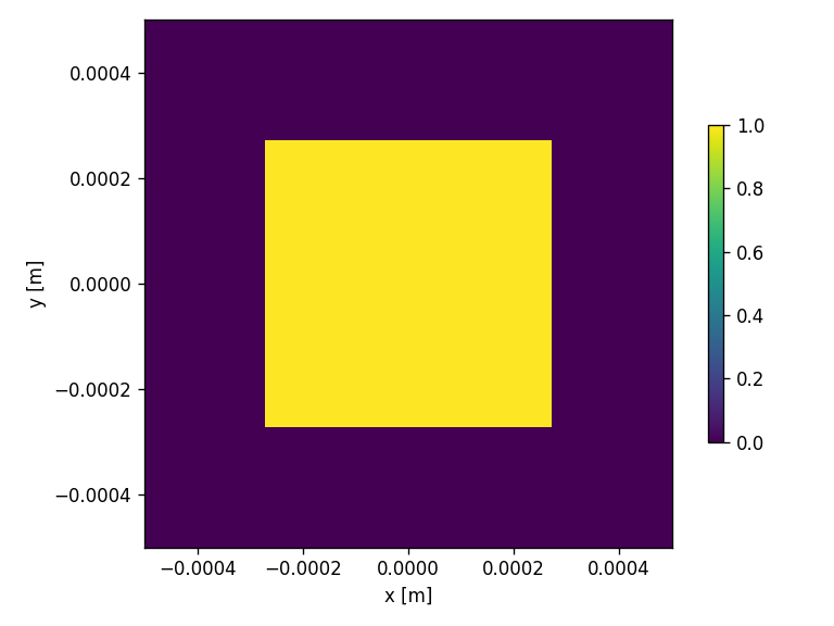
[29]:
# Make circular apertures (returns also the 2D array)
shape = (1024, 1024)
pad_width = (512, 512) # padding to linearize the FFT
spectrum = 0.532e-6 # wavelength
dxi = 2 * spectrum
D = dxi * shape[0] # field shape
w = D / 2 # width of aperture
z = 100 * D # propagation distance
spacing = dxi
n = 1 # refractive index of medium
wavelength = spectrum
zdist = z
pixsize = dxi
x_pixel = shape[0]
y_pixel = x_pixel
aperture_width = 1000e-6
aperture_height = 1000e-6
radius = 1000e-9 #m
#################################################################################################
# Make circular apertures (returns also the 2D array)
#wavelength = 500e-9 #m
N_box = 512
N_box = x_pixel
M_box = 8
L_box = 128e-6 #um
L_box = aperture_width
D_box = D/2
z_box = M_box / N_box / wavelength * L_box**2 * 2 #m
z_box = zdist
pixsize = L_box / N_box
x_pixel = N_box
y_pixel = N_box
aperture_width = x_pixel*pixsize
aperture_height = y_pixel*pixsize
y_box = np.linspace(-L_box/2, L_box/2, N_box, endpoint=False)
x_box = y_box
XX, YY =np.meshgrid(x_box, y_box)
print(np.shape(XX))
U_box = ((XX)**2 <= (D_box / 2)**2) * (YY**2 <= (D_box / 2)**2) *\
(np.exp(1j * np.pi / 2))
# Define Aperture
aperture = moe.generate.create_empty_aperture(-aperture_width/2, aperture_width/2, x_pixel, -aperture_height/2, aperture_height/2, y_pixel)
# Define Phase mask
mask_phase = moe.generate.create_empty_aperture_from_aperture(aperture)
mask_phase.aperture = np.angle(U_box)
mask_amplitude = moe.generate.create_empty_aperture_from_aperture(aperture)
mask_amplitude.aperture = np.abs(U_box)
# Plot the circular mask
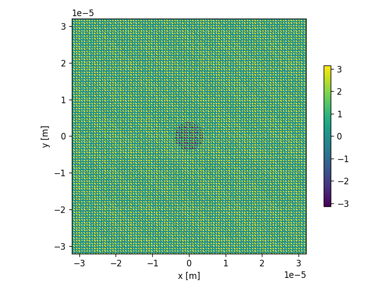
moe.plotting.plot_aperture(mask_phase)
moe.plotting.plot_aperture(mask_amplitude)
# Calculates a field to use with the calculated mask
# Initialize a Field from the Aperture mask
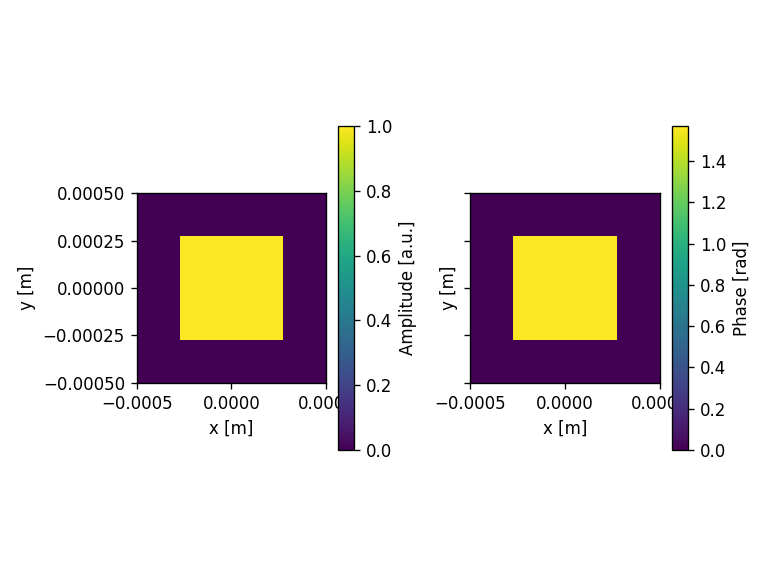
field = moe.field.create_empty_field_from_aperture(mask_phase)
# Generate a uniform field
field = moe.field.generate_uniform_field(field, E0=1)
# Modulates the field with a given aperture that can be used either as an amplitude mask or a phase mask
field = moe.field.modulate_field(field, amplitude_mask=mask_amplitude, phase_mask=mask_phase)
# Plots the field (amplitude and phase)
moe.plotting.plot_field(field)
plt.tight_layout()
plt.show()
(1024, 1024)
Propagate with ASM
[30]:
###Propagate field and calculate in plane YZ, using npix bins in Y
zmin = wavelength*200
zmax = zdist
nzs = 100

# Creates a screen in YZ plane with [-aperture_height/2, aperture_height/2] and [zmin, zmax] and
ymin, ymax = -aperture_height/2, aperture_height/2
xmin, xmax = -aperture_height/2, aperture_height/2

x = np.linspace(xmin, xmax, x_pixel)
y = np.linspace(ymin, ymax, y_pixel)
z = np.linspace(zmin, zmax, nzs)

screen = moe.Screen(x,y,z)

# Propagate the field
EXYZ = moe.propagate.ASM(field, screen, wavelength, pad=500, bl=True, mode="czt")


moe.plotting.plot_screen_YZ(EXYZ, which='amplitude')
plt.tight_layout()
plt.show()


moe.plotting.plot_screen_XY(EXYZ, z=zdist, which='amplitude')


moe.plotting.plot_screen_ZZ(EXYZ,x=0,y=0, which='amplitude')

plt.show()
ASM-CZT mode ON, with band limit.
Progress: [####################] 100.0%
Elapsed: 0:05:50.980069


Propagate with Bluestein
[31]:
#######################################################################################################
###Propagate field and calculate in plane YZ, using npix bins in Y
zmin = wavelength*200
zmax = zdist
nzs = 100
pad_factor=2
# Creates a screen in YZ plane with [-aperture_height/2, aperture_height/2] and [zmin, zmax] and
ymin, ymax = -aperture_height/2, aperture_height/2
xmin, xmax = -aperture_height/2, aperture_height/2
x = np.linspace(xmin, xmax, x_pixel)
y = np.linspace(ymin, ymax, y_pixel)
z = np.linspace(zmin, zmax, nzs)
screen = moe.Screen(x,y,z)
# Propagate the field
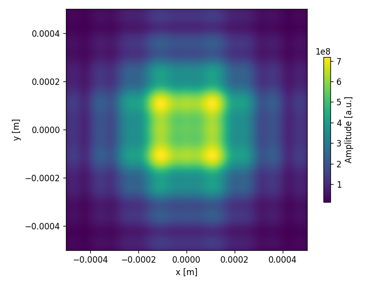
EXYZ = moe.propagate.Bluestein(field, screen, wavelength)#, pad_factor=pad_factor, crop = True)
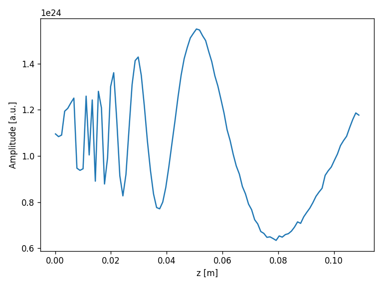
moe.plotting.plot_screen_XY(EXYZ, z=zdist, which='amplitude')
moe.plotting.plot_screen_ZZ(EXYZ,x=0,y=0, which='amplitude')
plt.ylim([0.2e9, 0.8e9])
limitx = moe.propagate.Fresnel_criterion(wavelength,radius)
plt.axvline(limitx, color='red', linestyle='dashed', lw=2)
plt.title("Valid for z > "+str(limitx))
plt.annotate("Fresnel distance", (1.4e-6,0.5e-6), rotation="vertical", color="Red")
plt.show()
moe.plotting.plot_screen_YZ(EXYZ,x=0, which='amplitude')
Progress: [####################] 100.0%
Elapsed: 0:01:41.618551
Propagate field and calculate in plane YZ, using npix bins in Y
[32]:
###Propagate field and calculate in plane YZ, using npix bins in Y
zmin = wavelength*200
zmax = zdist
nzs =4

# Creates a screen in YZ plane with [-aperture_height/2, aperture_height/2] and [zmin, zmax] and
ymin, ymax = -aperture_height/2, aperture_height/2
xmin, xmax = -aperture_height/2, aperture_height/2

x = np.linspace(xmin, xmax, x_pixel*3)
y = np.linspace(ymin, ymax, y_pixel*3)
z = np.linspace(zmin, zmax, nzs)

screen = moe.Screen(x,y,z)

# Propagate the field
EXYZ = moe.propagate.ASM(field, screen, wavelength, pad=1000, bl=False, mode=None)

moe.plotting.plot_screen_YZ(EXYZ, which='amplitude')
plt.tight_layout()

plt.show()

moe.plotting.plot_screen_XY(EXYZ, z=zdist, which='amplitude')
Conventional ASM, without band limit.
Progress: [####################] 100.0%
Elapsed: 0:00:31.973255

[33]:
EXYZ.screen.shape
[33]:
(3072, 3072, 4)
Band limited ASM
[34]:
###Propagate field and calculate in plane YZ, using npix bins in Y
zmin = wavelength*200
zmax = zdist
nzs =4

# Creates a screen in YZ plane with [-aperture_height/2, aperture_height/2] and [zmin, zmax] and
ymin, ymax = -aperture_height/2, aperture_height/2
xmin, xmax = -aperture_height/2, aperture_height/2

x = np.linspace(xmin, xmax, x_pixel*2)
y = np.linspace(ymin, ymax, y_pixel*2)
z = np.linspace(zmin, zmax, nzs)

screen = moe.Screen(x,y,z)

# Propagate the field
EXYZ = moe.propagate.ASM(field, screen, wavelength, pad=1000, mode="BLAS")

moe.plotting.plot_screen_YZ(EXYZ, which='amplitude')
plt.tight_layout()
plt.show()

moe.plotting.plot_screen_XY(EXYZ, z=zdist, which='amplitude')
BLAS mode ON.
Progress: [####################] 100.0%
Elapsed: 0:00:27.233123

ASM with Chirp Z-Transform
[35]:
###Propagate field and calculate in plane YZ, using npix bins in Y
zmin = wavelength*200
zmax = zdist
nzs =4

# Creates a screen in YZ plane with [-aperture_height/2, aperture_height/2] and [zmin, zmax] and
ymin, ymax = -aperture_height/2, aperture_height/2
xmin, xmax = -aperture_height/2, aperture_height/2

x = np.linspace(xmin, xmax, x_pixel*2)
y = np.linspace(ymin, ymax, y_pixel*2)
z = np.linspace(zmin, zmax, nzs)

screen = moe.Screen(x,y,z)

# Propagate the field
EXYZ = moe.propagate.ASM(field, screen, wavelength, pad=1000, bl=False, mode="czt")

moe.plotting.plot_screen_YZ(EXYZ, which='amplitude')
plt.tight_layout()

plt.show()

moe.plotting.plot_screen_XY(EXYZ, z=zdist, which='amplitude')
ASM-CZT mode ON, without band limit.
Progress: [####################] 100.0%
Elapsed: 0:00:32.074945
[36]:
###Propagate field and calculate in plane YZ, using npix bins in Y
zmin = wavelength*200
zmax = zdist
nzs =4

# Creates a screen in YZ plane with [-aperture_height/2, aperture_height/2] and [zmin, zmax] and
ymin, ymax = -aperture_height/2, aperture_height/2
xmin, xmax = -aperture_height/2, aperture_height/2

x = np.linspace(0, xmax, x_pixel*2)
y = np.linspace(0, ymax, y_pixel*2)
z = np.linspace(zmin, zmax, nzs)

screen = moe.Screen(x,y,z)

# Propagate the field
EXYZ = moe.propagate.ASM(field, screen, wavelength, pad=1000, bl=True, mode=None)


moe.plotting.plot_screen_YZ(EXYZ, which='amplitude')
plt.tight_layout()

plt.show()


moe.plotting.plot_screen_XY(EXYZ, z=zdist, which='amplitude')
Conventional ASM, with band limit.
Progress: [####################] 100.0%
Elapsed: 0:00:29.260332


[37]:
###Propagate field and calculate in plane YZ, using npix bins in Y
zmin = wavelength*200
zmax = zdist
nzs =4

# Creates a screen in YZ plane with [-aperture_height/2, aperture_height/2] and [zmin, zmax] and
ymin, ymax = -aperture_height/2, aperture_height/2
xmin, xmax = -aperture_height/2, aperture_height/2

x = np.linspace(0, xmax, x_pixel*2)
y = np.linspace(0, ymax, y_pixel*2)
z = np.linspace(zmin, zmax, nzs)

screen = moe.Screen(x,y,z)

# Propagate the field
EXYZ = moe.propagate.ASM(field, screen, wavelength, pad=1000, bl=True, mode="BLAS")


moe.plotting.plot_screen_YZ(EXYZ, which='amplitude')
plt.tight_layout()

plt.show()


moe.plotting.plot_screen_XY(EXYZ,z=zdist, which='amplitude')
BLAS mode ON.
Progress: [####################] 100.0%
Elapsed: 0:01:21.446096

[38]:
###Propagate field and calculate in plane YZ, using npix bins in Y
zmin = wavelength*200
zmax = zdist
nzs =4

# Creates a screen in YZ plane with [-aperture_height/2, aperture_height/2] and [zmin, zmax] and
ymin, ymax = -aperture_height/2, aperture_height/2
xmin, xmax = -aperture_height/2, aperture_height/2

x = np.linspace(0, xmax, x_pixel*2)
y = np.linspace(0, ymax, y_pixel*2)
z = np.linspace(zmin, zmax, nzs)

screen = moe.Screen(x,y,z)

# Propagate the field
EXYZ = moe.propagate.ASM(field, screen, wavelength, pad=1000, bl=True, mode="czt")


moe.plotting.plot_screen_YZ(EXYZ, which='amplitude')
plt.tight_layout()

plt.show()
moe.plotting.plot_screen_XY(EXYZ,z=zdist, which='amplitude')
ASM-CZT mode ON, with band limit.
Progress: [####################] 100.0%
Elapsed: 0:00:33.496301

Propagation with Scalable Angular Spectrum Method propagation
[39]:
###Propagate field and calculate in plane YZ, using npix bins in Y
zmin = wavelength*200
zmax = zdist
nzs =4

# Creates a screen in YZ plane with [-aperture_height/2, aperture_height/2] and [zmin, zmax] and
ymin, ymax = -aperture_height/2, aperture_height/2
xmin, xmax = -aperture_height/2, aperture_height/2

x = np.linspace(xmin, xmax, x_pixel)
y = np.linspace(ymin, ymax, y_pixel)
z = np.linspace(zmin, zmax, nzs)

screen = moe.Screen(x,y,z)

# Propagate the field
EXYZ = moe.propagate.SASM(field, screen, wavelength, pad_factor=2, crop = True)

moe.plotting.plot_screen_YZ(EXYZ, which='amplitude')
plt.tight_layout()
plt.show()


moe.plotting.plot_screen_XY(EXYZ,z=zdist, which='amplitude')
Progress: [####################] 100.0%
Elapsed: 0:00:14.239598

[40]:
###Propagate field and calculate in plane YZ, using npix bins in Y
zmin = wavelength*200
zmax = zdist
nzs =4

# Creates a screen in YZ plane with [-aperture_height/2, aperture_height/2] and [zmin, zmax] and
ymin, ymax = -aperture_height/2, aperture_height/2
xmin, xmax = -aperture_height/2, aperture_height/2

x = np.linspace(xmin, xmax, x_pixel)
y = np.linspace(ymin, ymax, y_pixel)
z = np.linspace(zmin, zmax, nzs)

screen = moe.Screen(x,y,z)

# Propagate the field
EXYZ = moe.propagate.ASM(field, screen, wavelength, pad = 2000, bl = True, mode="czt")

moe.plotting.plot_screen_YZ(EXYZ, which='amplitude')
plt.tight_layout()
plt.show()
moe.plotting.plot_screen_XY(EXYZ,z=zdist, which='amplitude')
ASM-CZT mode ON, with band limit.
Progress: [####################] 100.0%
Elapsed: 0:01:25.303954
Propagation from a Fresnel Zone Plate
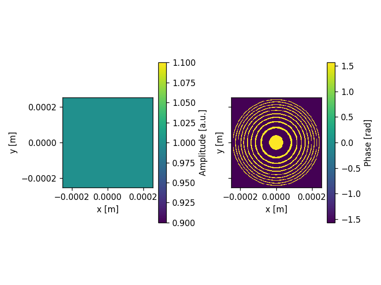
[41]:
#### Generate a fresnel zone plate

#number of pixels
x_pixel = 200
y_pixel = 200

#size of the rectangular mask
aperture_width  = 500e-6 #m
aperture_height = 500e-6

pixsize = aperture_width/x_pixel #m

wavelength = 632.8e-9 #m
focal_length = 5000e-6

zmin = wavelength
zmax = 1.2* focal_length
nzs = 256

radius = aperture_width/2

# Create Aperture
aperture1 = moe.generate.create_empty_aperture(-aperture_width/2, aperture_width/2, x_pixel, -aperture_height/2, aperture_height/2, y_pixel)

# Populate Aperture with Fresnel mask
mask1 = moe.generate.fresnel_phase(aperture1, focal_length, wavelength )

moe.plotting.plot_aperture(mask1)


##############
###Fresnel mask with a truncated circular aperture

# Create empty mask
aperture2 = moe.generate.create_empty_aperture_from_aperture(aperture1)

# and truncate around radius
mask2 = moe.generate.fresnel_phase(aperture2, focal_length, wavelength, radius=radius)
moe.plotting.plot_aperture(mask2)

# Discretize mask in number of levels
# Select exact position of contours  in phase
phase_vals = [ -np.pi/2, np.pi/2]

mask2.discretize(np.array( phase_vals)[:] )
moe.plotting.plot_aperture(mask2)


[42]:
# Generate a uniform field
field = moe.field.create_empty_field_from_aperture(mask2)

field = moe.field.generate_uniform_field(field, E0=1)

# Modulates the field
field = moe.field.modulate_field(field, amplitude_mask=None, phase_mask=mask2)

# Plots the field (amplitude and phase)
moe.plotting.plot_field(field)

plt.tight_layout()
plt.show()
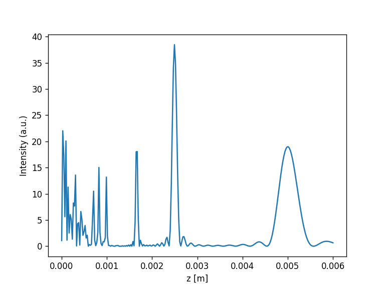
[43]:
# Propagates the field in a single line along the Z axis
screen_ZZ = moe.field.create_screen_ZZ(zmin, zmax, nzs)
E_ZZ = moe.propagate.RS_integral(field, screen_ZZ, wavelength)

# Get the intensity
I_ZZ = E_ZZ.amplitude[0,0,:]**2


# Plot the intensity
fig = plt.figure()

zp = np.linspace(zmin,zmax,nzs)

plt.plot(zp, I_ZZ)
plt.xlabel("z [m]")
plt.ylabel("Intensity (a.u.)")

plt.savefig("FZP-Zprop.png")
Warning: Sampling field pixel is larger than wavelength/2!
[########################################] | 100% Completed | 1.02 sms
Propagate with RS
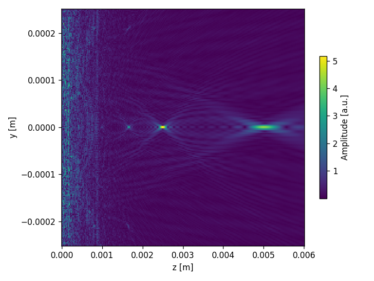
[44]:
#### Propagate field and calculate in plane YZ, using 100 bins in Y

nbins_y= x_pixel

# Creates YZ screen
screen_YZ = moe.field.create_screen_YZ(-aperture_height/2, aperture_height/2, nbins_y,
                                        zmin, zmax, nzs,
                                        x=0)

# Propagate the field
E_YZ = moe.propagate.RS_integral(field, screen_YZ, wavelength, simp2d=True)
Warning: Sampling field pixel is larger than wavelength/2!
[########################################] | 100% Completed | 135.52 s
[45]:
#Plot the amplitude of the propagated field in yz screen
moe.plotting.plot_screen_YZ(E_YZ, which='amplitude')

plt.savefig("FresnelN2-YZ.png")

plt.show()
Propagate with Bluestein
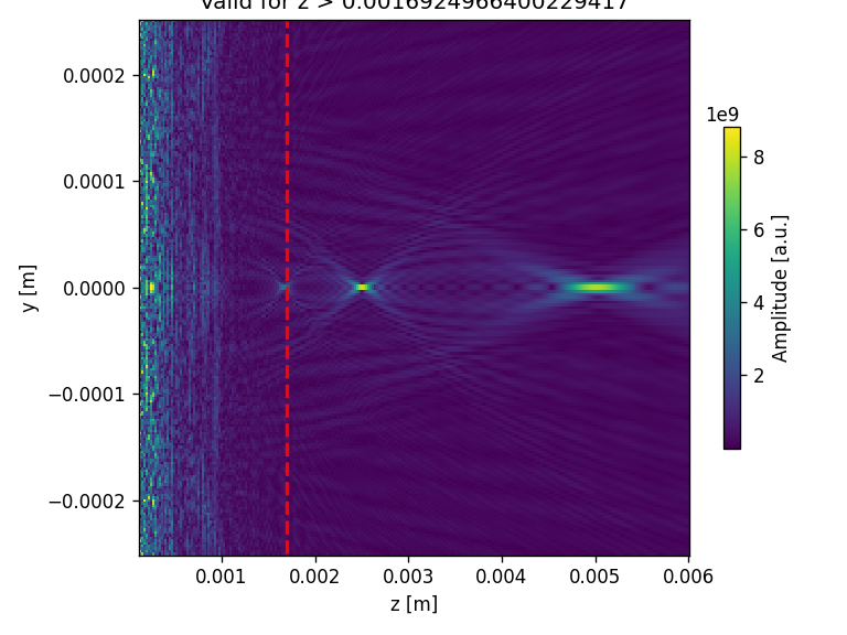
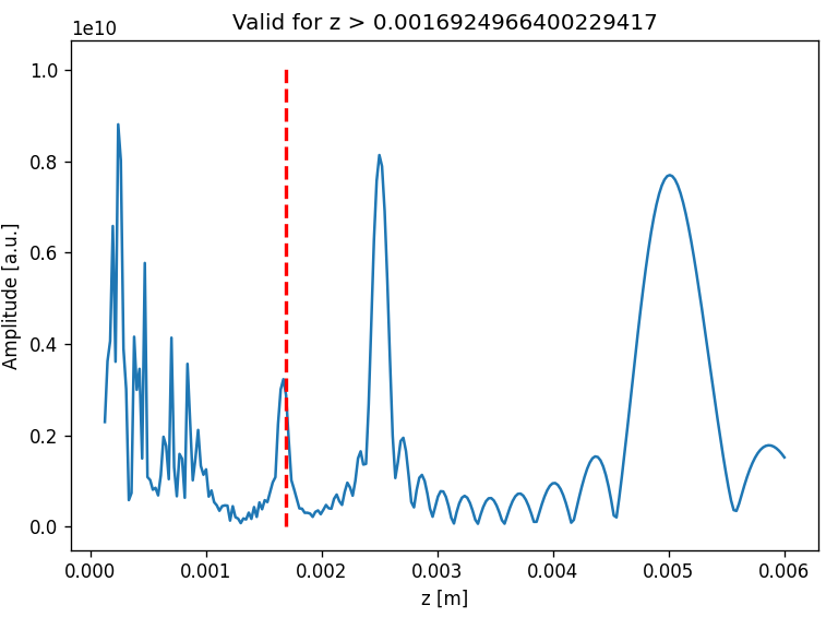
[46]:
# Propagate via Bluestein

# Creates a screen in YZ plane with [-aperture_height/2, aperture_height/2] and [zmin, zmax] and
ymin, ymax = -aperture_height/2, aperture_height/2
xmin, xmax = -aperture_width/2, aperture_width/2

x = np.linspace(xmin, xmax, x_pixel)
y = np.linspace(ymin, ymax, y_pixel)
z = np.linspace(zmin*200, zmax, nzs)


screen = moe.Screen(x,y,z)

# Propagate the field
EXYZ = moe.propagate.Bluestein(field, screen, wavelength)

moe.plotting.plot_screen_YZ(EXYZ, which='amplitude')

limitx = moe.propagate.Fresnel_criterion(wavelength,radius)
plt.vlines(limitx, -radius, radius, colors='red', linestyles='dashed', lw=2)

plt.title("Valid for z > "+str(limitx))

plt.show()

moe.plotting.plot_screen_XY(EXYZ, z=focal_length, which='amplitude')

moe.plotting.plot_screen_ZZ(EXYZ, which='amplitude')

limitx = moe.propagate.Fresnel_criterion(wavelength,radius)
plt.vlines(limitx, 0, np.max(EXYZ.screen), colors='red', linestyles='dashed', lw=2)

plt.title("Valid for z > "+str(limitx))

plt.show()
Progress: [####################] 100.0%
Elapsed: 0:00:06.763499
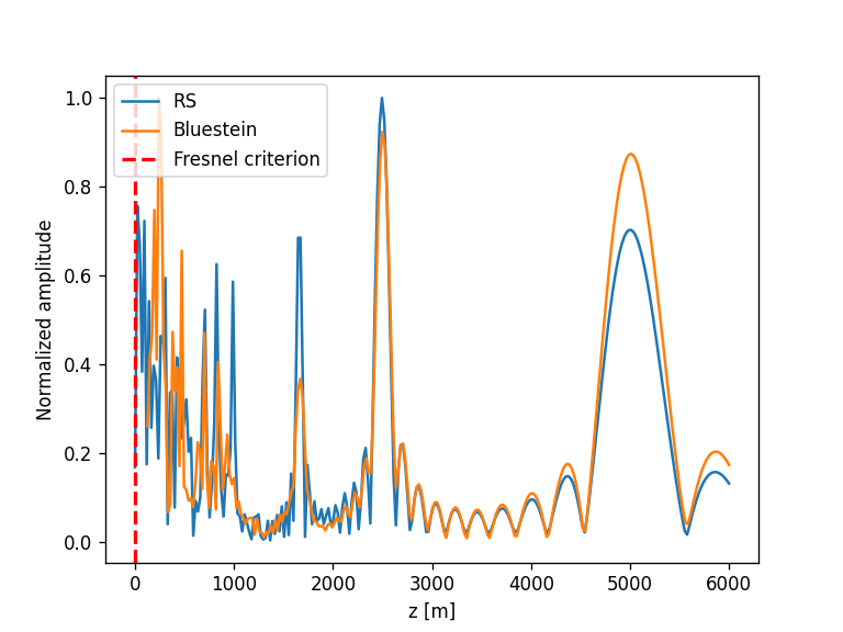
Compare RS and Bluestein propagations
[47]:
fig = plt.figure()

zRS = screen_ZZ.z/scale
amplitudeRS = np.abs(screen_ZZ.slice_Z(0,0))
phaseRS = np.angle(screen_ZZ.slice_Z(0,0))

zBS = EXYZ.z/scale
amplitudeBS = np.abs(EXYZ.slice_Z(0,0))
phaseBS = np.angle(EXYZ.slice_Z(0,0))

fig = plt.figure()

plt.plot(zRS, amplitudeRS/np.max(amplitudeRS), label="RS")
plt.plot(zBS, amplitudeBS/np.max(amplitudeBS), label="Bluestein")
plt.axvline(limitx, color='red', linestyle='dashed', lw=2, label='Fresnel criterion')

plt.legend()

plt.xlabel("z [m]")
plt.ylabel("Normalized amplitude")
[47]:
Text(0, 0.5, 'Normalized amplitude')
<Figure size 768x576 with 0 Axes>
Spiral Phase Plate
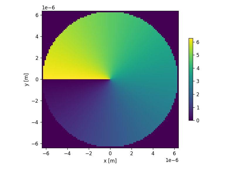
[48]:
### Spiral Phase plate

npix = 100 # nr of pixels

wavelength = 632.8e-9 #wavelength in m
z_distance = 100*wavelength # propagation distance

aperture_width = 20*wavelength  #x-size in m
aperture_height = 20*wavelength #y-size in m

pixsize = aperture_width/npix

ltop = 1 #topological number

#spiral mask is defined as
#spiral(x,y,x0,y0,ltop)

def spiral(x,y,x0,y0,L):
    """
    returns a spiral COMPLEX PHASE with input meshgrid (x,y) with center at (x0,y0)
    x = x array from meshgrid
    y = y array from meshgrid
    x0 = x-coordinate of center of the lens
    y0 = y-coordinate of center of the lens
    L = topological charge
    """

    theta = np.arctan2((y-y0),(x-x0))
    sp = np.exp(1.0j*L*theta)
    return sp


n =10 # number of gray levels

center = (0, 0)

aperture = moe.generate.create_empty_aperture(-aperture_width/2, aperture_width/2, npix, -aperture_height/2, aperture_height/2, npix)
mask =  moe.generate.arbitrary_aperture_function(aperture, moe.sag.spiral, center=center, L=ltop)
mask.aperture = mask.aperture + np.pi

mask.aperture[np.where(mask.XX**2+mask.YY**2>(aperture_width/2)**2 ) ] = 0
moe.plotting.plot_aperture(mask)
[49]:
# Generate a uniform field
field = moe.field.create_empty_field_from_aperture(mask)

field = moe.field.generate_uniform_field(field, E0=1)

aperture = moe.generate.create_empty_aperture_from_aperture(mask)

mask_circle = moe.generate.circular_aperture(aperture, radius=aperture_width/2)

# Modulates the field
field = moe.field.modulate_field(field, amplitude_mask=mask_circle, phase_mask=mask)

# Plots the field (amplitude and phase)
moe.plotting.plot_field(field)

plt.tight_layout()
plt.show()
[50]:
##Propagate field in plane XY at z_distance

# Creates XY screen
screen_XY = moe.field.create_screen_XY(-aperture_width/2, aperture_width/2, npix,
                                       -aperture_height/2, aperture_height/2, npix,
                                        z=z_distance)

# Propagate the field
E_XY = moe.propagate.RS_integral(field, screen_XY, wavelength, simp2d=True)
[########################################] | 100% Completed | 23.85 s
[51]:
# Plot the amplitude of the propagated field in XY screen

moe.plotting.plot_screen_XY(E_XY)
#plt.title("z = "+str(z_distance)+" m")

plt.tight_layout()
plt.savefig("Spiral-N16-XY.png")

plt.show()
[52]:
#### Propagate field and calculate in plane YZ

nbins_y = x_pixel
zmin = wavelength
zmax = 2 * z_distance
nzs = 500

# Creates YZ screen
screen_YZ = moe.field.create_screen_YZ(-aperture_height/2, aperture_height/2, nbins_y,
                                        zmin, zmax, nzs,
                                        x=0)

# Propagate the field
E_YZ = moe.propagate.RS_integral(field, screen_YZ, wavelength, simp2d=True)
[########################################] | 100% Completed | 235.04 s
[53]:
#Plot the amplitude of the propagated field in yz screen
moe.plotting.plot_screen_YZ(E_YZ, which='amplitude')

plt.savefig("Spiral-YZ.png")

plt.show()
Alvarez Lenses Pair
[54]:
# Creates an Alvarez lens pair masks
# evaluates the produced focal spot by the displaced lenses using the propagation
aperture_width = 1000*micro
aperture_height = 500*micro
x_pixel = 1000
y_pixel = 500


# focal range of the Alvarez lenses
f1 = 500*micro
f2 = 15000*micro
tuning_distance = 100*micro
wavelength = 1550*nano

#nr of levels
n = 8

# First lens
aperture = moe.generate.create_empty_aperture(-aperture_width/2, aperture_width/2, x_pixel, -aperture_height/2, aperture_height/2, y_pixel,)
lens1 =  moe.generate.arbitrary_aperture_function(aperture, moe.sag.Alvarez_phase, f1=f1, f2=f2, tuning_distance=tuning_distance, wavelength=wavelength)

lens1.modulos(2*np.pi)
lens1.discretize(n)

# Second lens which is the same but flipped.
aperture2 = moe.generate.create_empty_aperture(-aperture_width/2, aperture_width/2, x_pixel, -aperture_height/2, aperture_height/2, y_pixel,)

lens2 =  moe.generate.arbitrary_aperture_function(aperture2, moe.sag.Alvarez_phase, f1=f1, f2=f2, tuning_distance=tuning_distance, wavelength=wavelength)

lens2.aperture = np.flipud(lens2.aperture)

lens2.modulos(2*np.pi)
lens2.discretize(n)

# initializes an aperture to store the result
result = moe.generate.create_empty_aperture(-aperture_width/2, aperture_width/2, x_pixel, -aperture_height/2, aperture_height/2, y_pixel,)


# displace aperture equally both ways, total displacement is twice displacement
displacement = 12*micro
rollidx = int(np.round(displacement/lens1.pixel_x,))

roll = rollidx
lens1.aperture = np.roll(lens1.aperture, -roll, axis=0)
lens2.aperture = np.roll(lens2.aperture, roll, axis=0)

lens1.aperture[-roll:,0] = 0
lens2.aperture[:roll, 0] = 0


# Calculates the resulting aperutre by the sum of both displaced lens1 and lens2
result.aperture = -lens1.aperture - lens2.aperture

result.modulos(2*np.pi)
[55]:
# Creates a mask from the result, and modulates the phase of a gaussian field

mask = result
field = moe.field.create_empty_field_from_aperture(mask)
field = moe.field.generate_gaussian_field(field, E0=1, w0=400*micro)

field = moe.field.modulate_field(field, amplitude_mask=None, phase_mask=result)

moe.plotting.plot_field(field)
[56]:
screen_YZ = moe.field.create_screen_YZ(-250*micro,250*micro, 101, 100*micro, 10000*micro, 101)
E_YZ = moe.propagate.RS_integral(field, screen_YZ, wavelength, )#method="trap")

moe.plotting.plot_screen_YZ(E_YZ, which='amplitude')
Warning: Sampling field pixel is larger than wavelength/2!
[########################################] | 100% Completed | 459.24 s
[57]:
screen_ZZ = moe.field.create_screen_ZZ(100*micro, 10000*micro, 201)
E_ZZ = moe.propagate.RS_integral(field, screen_ZZ, wavelength,)

moe.plotting.plot_screen_ZZ(E_ZZ, which='amplitude')
Warning: Sampling field pixel is larger than wavelength/2!
[########################################] | 100% Completed | 9.56 ss
[58]:
screen_XY = moe.field.create_screen_XY(-50*micro,50*micro, 31,
                                        -50*micro,50*micro, 31,
                                        z=4150*micro)

E_XY = moe.propagate.RS_integral(field, screen_XY, wavelength)

moe.plotting.plot_screen_XY(E_XY)
Warning: Sampling field pixel is larger than wavelength/2!
[########################################] | 100% Completed | 44.17 s
[59]:
# Creates a screen in YZ plane with [-aperture_height/2, aperture_height/2] and [zmin, zmax] and
ymin, ymax = -250*micro,250*micro
xmin, xmax = -500*micro,500*micro


zmin, zmax, nzs = 100*micro, 10000*micro, 201

x = np.linspace(xmin, xmax, 1000)
y = np.linspace(ymin, ymax, 500)
z = np.linspace(zmin, zmax, nzs)

focal_length = 4150*micro


screen = moe.Screen(x,y,z)

# Propagate the field
EXYZ = moe.propagate.Bluestein(field, screen, wavelength)
Progress: [####################] 100.0%
Elapsed: 0:01:26.811377
[60]:
moe.plotting.plot_screen_YZ(EXYZ, which='amplitude')
plt.tight_layout()
plt.show()
moe.plotting.plot_screen_YZ(EXYZ, which='phase')
[61]:
moe.plotting.plot_screen_ZZ(EXYZ,x=0,y=0, which='amplitude')

radius= ymax
limitx = moe.propagate.Fresnel_criterion(wavelength,radius)
plt.vlines(limitx, 0, np.max(EXYZ.screen), colors='red', linestyles='dashed', lw=2)

plt.title("Valid for z > "+str(limitx))

plt.show()
Compare RS and Bluestein
[62]:
fig = plt.figure()

scale = 1
zRS = screen_ZZ.z/scale
amplitudeRS = np.abs(screen_ZZ.slice_Z(0,0))
phaseRS = np.angle(screen_ZZ.slice_Z(0,0))

zBS = EXYZ.z/scale
amplitudeBS = np.abs(EXYZ.slice_Z(0,0))
phaseBS = np.angle(EXYZ.slice_Z(0,0))

fig = plt.figure()

plt.plot(zRS, amplitudeRS/np.max(amplitudeRS), label="RS")
plt.plot(zBS, amplitudeBS/np.max(amplitudeBS), label="Bluestein")
plt.axvline(limitx, color='red', linestyle='dashed', lw=2, label='Fresnel criterion')

plt.legend()

plt.xlabel("z [m]")
plt.ylabel("Normalized amplitude")
[62]:
Text(0, 0.5, 'Normalized amplitude')
<Figure size 768x576 with 0 Axes>
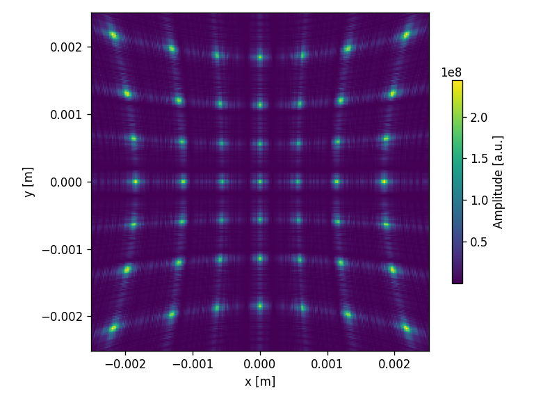
Dammann Gratings
2D Dammann Grating
[63]:
# Generates and propagates a Dammann grating phase

aperture_width = 100*micro
aperture_height = 100*micro
x_pixel = 100
y_pixel = 100

aperture = moe.generate.create_empty_aperture(-aperture_width/2, aperture_width/2, x_pixel, -aperture_height/2, aperture_height/2, y_pixel,)


transitions_x = [0.242, 0.414]
transitions_y = [0.242, 0.414]


period_x = period_y = 10*micro


mask =  moe.generate.arbitrary_aperture_function(aperture, moe.sag.dammann_2d, transitions_x=transitions_x, period_x=period_x, transitions_y=transitions_y, period_y=period_y)

mask.aperture = mask.aperture*np.pi/2 + np.pi/2

aperture2 = moe.generate.create_empty_aperture(-aperture_width/2+50*aperture.pixel_x, \
                                              aperture_width/2+50*aperture.pixel_x, x_pixel+500, \
                                              -aperture_height/2+50*aperture.pixel_y, \
                                              aperture_height/2+50*aperture.pixel_y, y_pixel+500,)


aperture2.aperture = mask.aperture

moe.plotting.plot_aperture(mask)
[64]:
aperture = moe.generate.create_empty_aperture(-aperture_width/2, aperture_width/2, len(aperture.x), \
                                              -aperture_height/2, aperture_height/2, len(aperture.y),)
aperture.aperture = aperture2.aperture

field = moe.field.create_empty_field_from_aperture(aperture)
field = moe.field.generate_uniform_field(field, E0=1)
#field = moe.field.generate_gaussian_field(field, E0=1, w0=400*micro)

field = moe.field.modulate_field(field, amplitude_mask=None, phase_mask=aperture)


moe.plotting.plot_field(field)
[65]:
# define the wavelength used in the propagation
wavelength = 1550*nano

# Define the screen size and create it
screen_width = 5000*micro
screen_height = 5000*micro
x_pixel = 125
y_pixel = 125

screen_XY = moe.field.create_screen_XY(-screen_width/2, screen_width/2, x_pixel,
                                     -screen_height/2, screen_height/2, y_pixel,
                                     z=3500*micro)
Propagation with RS integral
Shows distortion
[66]:
#propagate with RS
E_XY = moe.propagate.RS_integral(field, screen_XY, wavelength)
Warning: Sampling field pixel is larger than wavelength/2!
[########################################] | 100% Completed | 47.94 s
[67]:
Exy_init = E_XY
[68]:
moe.plotting.plot_screen_XY(Exy_init, which='amplitude')
moe.plotting.plot_screen_XY(Exy_init, which='phase')

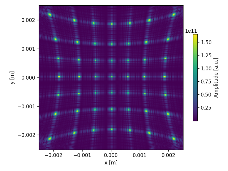
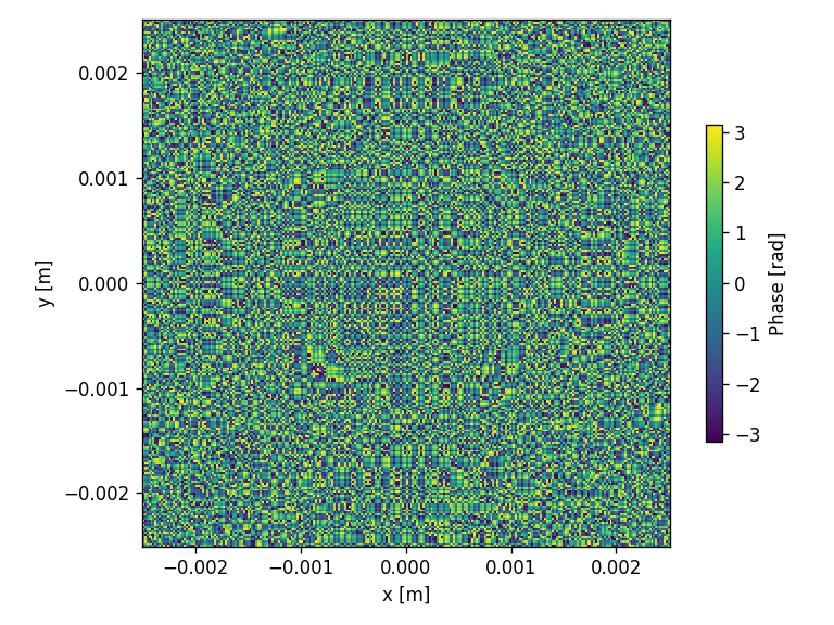
Propagation with ASM method
Shows distortion
[69]:
x = np.linspace(-screen_width/2, screen_width/2, 256)
y = np.linspace(-screen_height/2, screen_height/2, 256)
#z = np.linspace(wavelength, 3500*micro, 100)
z = [3500*micro] #[3500*micro]

screenx = moe.Screen(x,y,z)


#propagate with ASM
E_XY2 = moe.propagate.ASM(field, screenx, wavelength, pad=3000, bl=True, mode="czt")

moe.plotting.plot_screen_XY(E_XY2, which='amplitude')
moe.plotting.plot_screen_XY(E_XY2, which='phase')
ASM-CZT mode ON, with band limit.
Progress: [####################] 100.0%
Elapsed: 0:00:28.074955
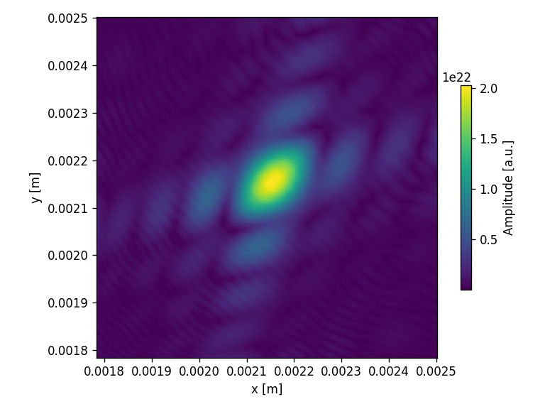
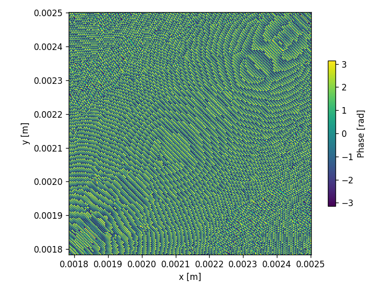
Simulation of a subsection of the image plane
[70]:
x = np.linspace(screen_width/2  - screen_width/7, screen_width/2, 256)
y = np.linspace(screen_height/2 - screen_height/7, screen_height/2, 256)
#z = np.linspace(wavelength, 3500*micro, 100)
z = [3500*micro] #[3500*micro]

screenx = moe.Screen(x,y,z)

#propagate with ASM
E_XY2 = moe.propagate.ASM(field, screenx, wavelength,3000, bl=True, mode="czt")

moe.plotting.plot_screen_XY(E_XY2, which='amplitude')
moe.plotting.plot_screen_XY(E_XY2, which='phase')
ASM-CZT mode ON, with band limit.
Progress: [####################] 100.0%
Elapsed: 0:00:27.655182
ASM with CZT
[71]:
x = np.linspace(-screen_width/2, screen_width/2, 256)
y = np.linspace(-screen_height/2, screen_height/2, 256)
#z = np.linspace(wavelength, 3500*micro, 100)
z = [3500*micro] #[3500*micro]

screenx = moe.Screen(x,y,z)


#propagate with ASM-CZT
E_XY2 = moe.propagate.ASM(field, screenx, wavelength, pad=3000, bl=True, mode="czt")

moe.plotting.plot_screen_XY(E_XY2, which='amplitude')
moe.plotting.plot_screen_XY(E_XY2, which='phase')
ASM-CZT mode ON, with band limit.
Progress: [####################] 100.0%
Elapsed: 0:00:28.050375


ASM with band limits
[72]:
x = np.linspace(-screen_width/2, screen_width/2, 256)
y = np.linspace(-screen_height/2, screen_height/2, 256)
#z = np.linspace(wavelength, 3500*micro, 100)
z = [3500*micro] #[3500*micro]

screenx = moe.Screen(x,y,z)


#propagate with ASM - BLAS
E_XY2 = moe.propagate.ASM(field, screenx, wavelength, pad = 2500, bl=True, mode="BLAS")

moe.plotting.plot_screen_XY(E_XY2, which='amplitude')
moe.plotting.plot_screen_XY(E_XY2, which='phase')
BLAS mode ON.
Progress: [####################] 100.0%
Elapsed: 0:01:02.223026
[73]:
x = np.linspace(-screen_width/2, screen_width/2, 256)
y = np.linspace(-screen_height/2, screen_height/2, 256)
#z = np.linspace(wavelength, 3500*micro, 100)
z = [3500*micro] #[3500*micro]

screenx = moe.Screen(x,y,z)


#propagate with ASM
E_XY2 = moe.propagate.ASM(field, screenx, wavelength, pad=2500, bl=True, mode=None)

moe.plotting.plot_screen_XY(E_XY2, which='amplitude')
moe.plotting.plot_screen_XY(E_XY2, which='phase')
Conventional ASM, with band limit.
Progress: [####################] 100.0%
Elapsed: 0:00:24.434535
Propagation with Scalable ASM
[74]:
x = np.linspace(-screen_width/2, screen_width/2, 256)
y = np.linspace(-screen_height/2, screen_height/2, 256)
#z = np.linspace(wavelength, 3500*micro, 100)
z = [3500*micro] #[3500*micro]

screenx = moe.Screen(x,y,z)


#propagate with SASM
E_XY2 = moe.propagate.SASM(field, screenx, wavelength, pad_factor = 13, crop = True)

moe.plotting.plot_screen_XY(E_XY2, which='amplitude')
moe.plotting.plot_screen_XY(E_XY2, which='phase')
Progress: [####################] 100.0%
Elapsed: 0:00:01.482623
Propagation with Bluestein
Fails to observe distortion!
[75]:
x = np.linspace(-screen_width/2, screen_width/2, 256)
y = np.linspace(-screen_height/2, screen_height/2, 256)
z = [3500*micro]

screenx = moe.Screen(x,y,z)

screen_XY2 = screenx

#propagate with bluestein
E_XY2 = moe.propagate.Bluestein(field, screenx, wavelength)

moe.plotting.plot_screen_XY(E_XY2, which='amplitude')
moe.plotting.plot_screen_XY(E_XY2, which='phase')
Progress: [####################] 100.0%
Elapsed: 0:00:00.030895

Distortion correction via coordinate transformation
[76]:
E_XY2_corrected = moe.propagate.distortion_correction(E_XY2.screen, E_XY2.x, E_XY2.y, E_XY2.z[-1], wavelength)

E_XY2.screen = E_XY2_corrected

moe.plotting.plot_screen_XY(E_XY2, which='amplitude')
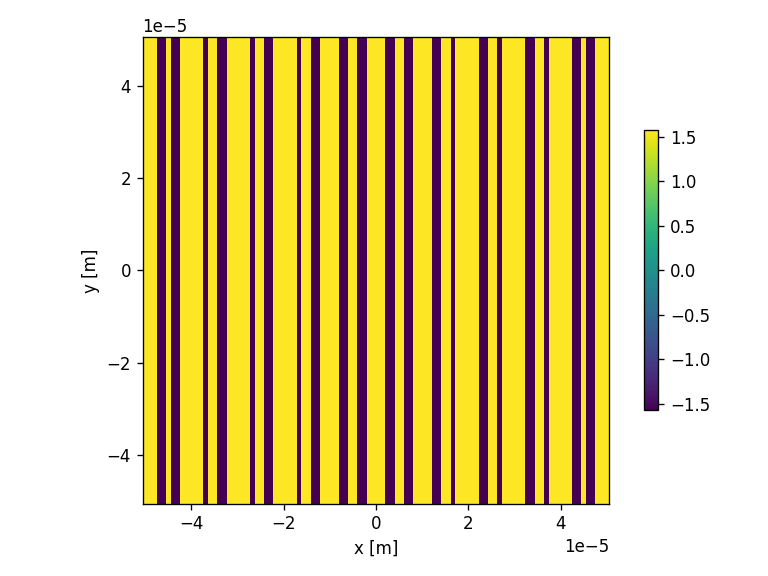
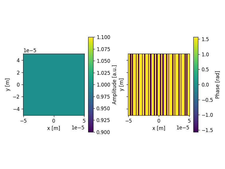
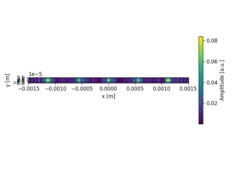
1D Dammann Grating
[76]:
# Generates and propagates a Dammann grating phase

aperture_width = 100*micro
aperture_height = 100*micro
x_pixel = 100
y_pixel = 100

aperture = moe.generate.create_empty_aperture(-aperture_width/2, aperture_width/2, x_pixel, -aperture_height/2, aperture_height/2, y_pixel,)


transitions_x = [0.132, 0.48]
transitions_x = [0.242, 0.414]
#transitions_x = [0.1, 0.136,0.37, 0.498]
#transitions_y = [0.1, 0.3]
transitions_y = None

period_x = period_y = 10*micro

# mask =  moe.generate.arbitrary_aperture_function(aperture, moe.sag.dammann_2d, L=L)
mask =  moe.generate.arbitrary_aperture_function(aperture, moe.sag.dammann_2d, transitions_x=transitions_x, period_x=period_x, transitions_y=transitions_y, period_y=period_y)

mask.aperture = mask.aperture*np.pi/2


moe.plotting.plot_aperture(mask)


field = moe.field.create_empty_field_from_aperture(mask)
field = moe.field.generate_uniform_field(field, E0=1)
# field = moe.field.modulate_field(field, amplitude_mask=mask, phase_mask=None)
field = moe.field.modulate_field(field, amplitude_mask=None, phase_mask=mask)


moe.plotting.plot_field(field)
[77]:
# define the wavelength used in the propagation
wavelength = 1550*nano

# Define the screen size and create it
screen_width = 3000*micro
screen_height = 3000*micro
x_pixel =256
y_pixel = 256

screen_XY = moe.field.create_screen_XY(-screen_width/2, screen_width/2, x_pixel,
                                     -screen_height/2, screen_height/2, y_pixel,
                                     z=3500*micro)

E_XY = moe.propagate.RS_integral(field, screen_XY, wavelength)

moe.plotting.plot_screen_XY(E_XY, which='amplitude')
plt.ylim(-aperture_height/2, aperture_height/2)
Warning: Sampling field pixel is larger than wavelength/2!
[########################################] | 100% Completed | 239.88 s
[77]:
(-4.9999999999999996e-05, 4.9999999999999996e-05)
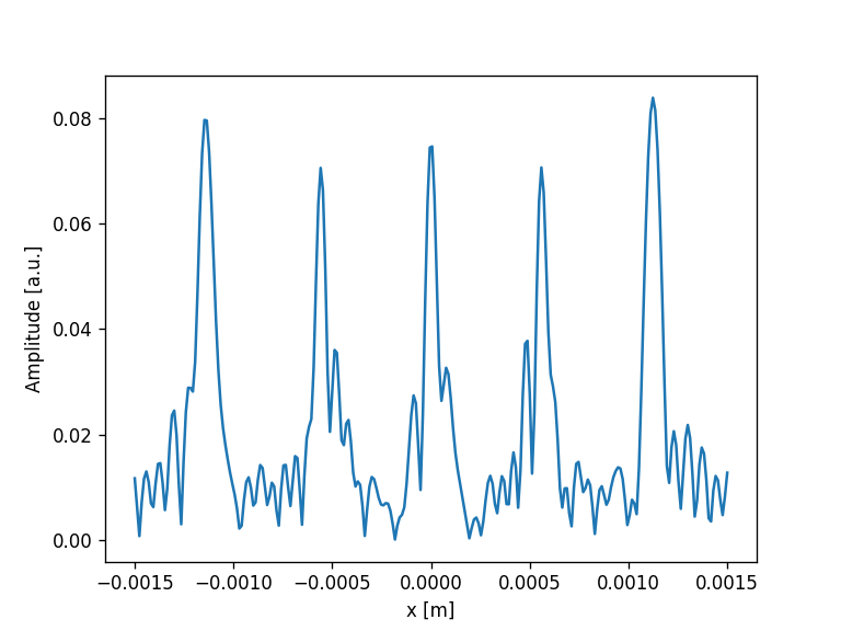
[78]:
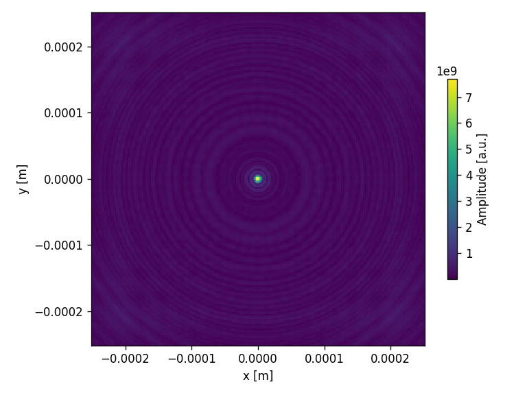
fig = plt.figure()

xmat= E_XY.amplitude[:,:,0]
y= xmat[:, int(xmat.shape[0]/2)]
x = E_XY.x

plt.plot(x,y)
plt.xlabel("x [m]")
plt.ylabel("Amplitude [a.u.]")
[78]:
Text(0, 0.5, 'Amplitude [a.u.]')
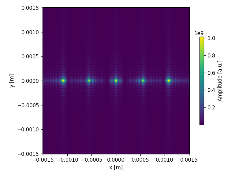
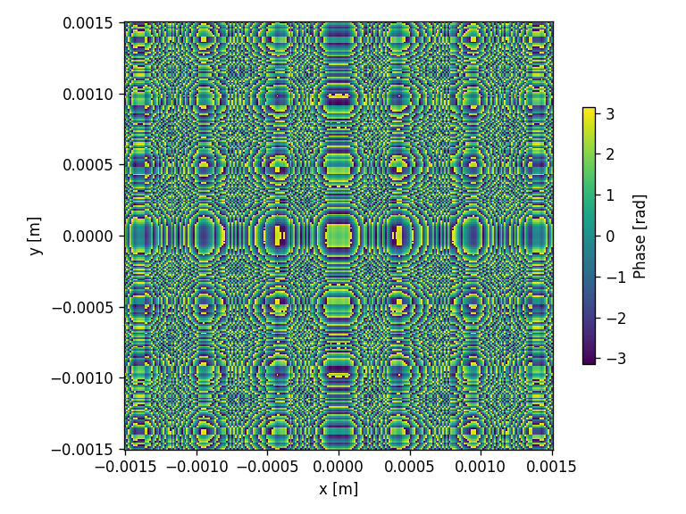
[79]:
# define the wavelength used in the propagation
wavelength = 1550*nano

screen_width = 3000*micro
screen_height = 3000*micro
x_pixel =256
y_pixel = 256

screen_XY = moe.field.create_screen_XY(-screen_width/2, screen_width/2, x_pixel,
                                     -screen_height/2, screen_height/2, y_pixel,
                                     z=3500*micro)

E_XY2 = moe.propagate.Bluestein(field, screen_XY, wavelength)

moe.plotting.plot_screen_XY(E_XY2, which='amplitude')
moe.plotting.plot_screen_XY(E_XY2, which='phase')
Progress: [####################] 100.0%
Elapsed: 0:00:00.027920
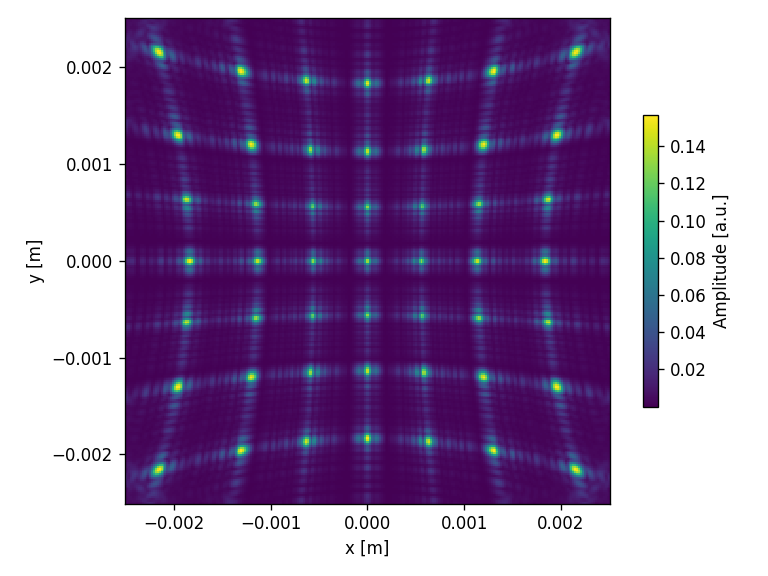
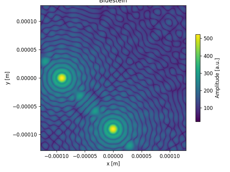
Angular Spectrum Method and Scalable Angular Spectrum Method Validation
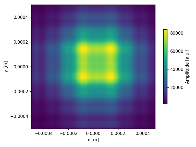
Check https://opg.optica.org/optica/fulltext.cfm?uri=optica-10-11-1407
[80]:
wavelength = 500e-9 #m
N_box =512
M_box =8
L_box = 128e-6 #um
D_box = L_box / 16
z_box = M_box / N_box / wavelength * L_box**2 * 2 #m
pixsize = L_box / N_box
x_pixel = N_box
y_pixel = N_box
aperture_width = x_pixel*pixsize
aperture_height = y_pixel*pixsize
y_box = np.linspace(-L_box/2, L_box/2, N_box, endpoint=False)
x_box = y_box
XX, YY =np.meshgrid(x_box, y_box, indexing='ij')
print(np.shape(XX))
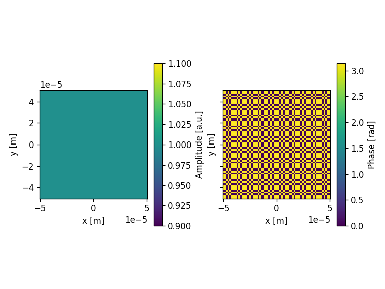
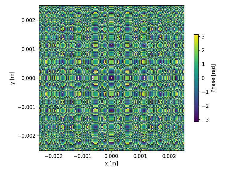
U_box = ((XX)**2 <= (D_box / 2)**2) * (YY**2 <= (D_box / 2)**2) *\
(np.exp(1j * 2 * np.pi / wavelength * XX * np.sin(20/ 360 * 2 * np.pi)))
# Define Aperture
aperture = moe.generate.create_empty_aperture(-aperture_width/2, aperture_width/2, x_pixel, -aperture_height/2, aperture_height/2, y_pixel)
# Define Phase mask
mask_phase = moe.generate.create_empty_aperture_from_aperture(aperture)
mask_phase.aperture = np.angle(U_box)
mask_amplitude = moe.generate.create_empty_aperture_from_aperture(aperture)
mask_amplitude.aperture = np.abs(U_box)
# Plot the circular mask
moe.plotting.plot_aperture(mask_phase)
moe.plotting.plot_aperture(mask_amplitude)
# Calculates a field to use with the calculated mask
# Initialize a Field from the Aperture mask
field = moe.field.create_empty_field_from_aperture(mask_phase)
# Generate a uniform field
field = moe.field.generate_uniform_field(field, E0=1)
# Modulates the field with a given aperture that can be used either as an amplitude mask or a phase mask
field = moe.field.modulate_field(field, amplitude_mask=mask_amplitude, phase_mask=mask_phase)
# Plots the field (amplitude and phase)
moe.plotting.plot_field(field)
plt.tight_layout()
plt.show()
(512, 512)

[81]:
###Propagate field and calculate in plane YZ, using npix bins in Y
zmin = wavelength*2
zmax = 1.2*z_box
nzs = 2
# Creates a screen in YZ plane with [-aperture_height/2, aperture_height/2] and [zmin, zmax] and
ymin, ymax = -aperture_height/2*10, aperture_height/2*10
xmin, xmax = -aperture_height/2*10, aperture_height/2*10
x = np.linspace(xmin, xmax, x_pixel)
y = np.linspace(ymin, ymax, y_pixel)
z = np.linspace(zmin, zmax, nzs)
screen = moe.Screen(x,y,z)
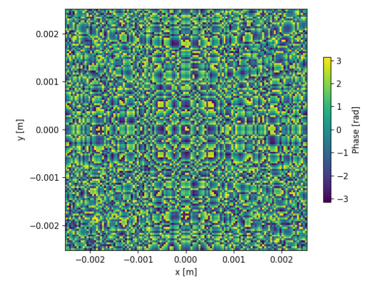
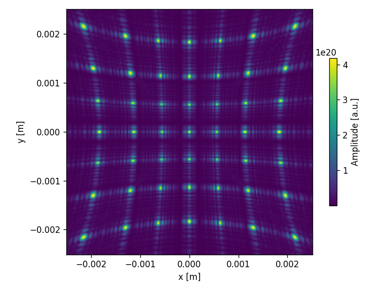
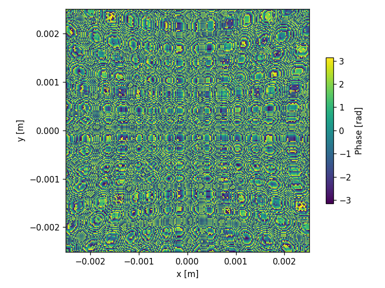
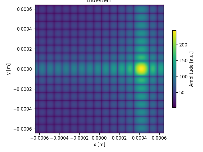
# Propagate the field with Bluestein
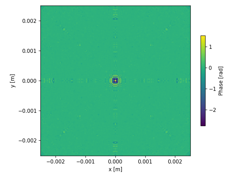
EXYZ = moe.propagate.Bluestein(field, screen, wavelength)
EXYZ.screen = (np.abs(0.0 + EXYZ.screen)**2)**0.13
moe.plotting.plot_screen_XY(EXYZ, z=z_box, which='amplitude')
plt.title("Bluestein")
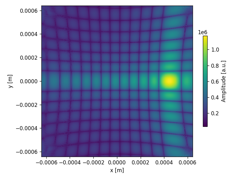
# Propagate the field with SASM
screen = moe.Screen(x,y,z)
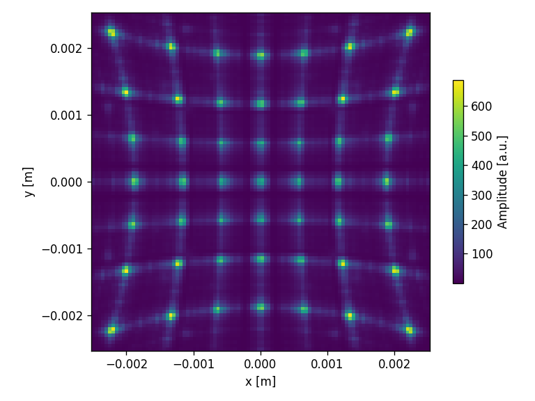
EXYZ = moe.propagate.SASM(field, screen, wavelength, pad_factor=2, crop=True)
EXYZ.screen = (np.abs(0.0 + EXYZ.screen)**2)**0.13
moe.plotting.plot_screen_XY(EXYZ, z=z_box, which='amplitude')
plt.title("SASM")
# Propagate the field with SASM
screen = moe.Screen(x,y,z)
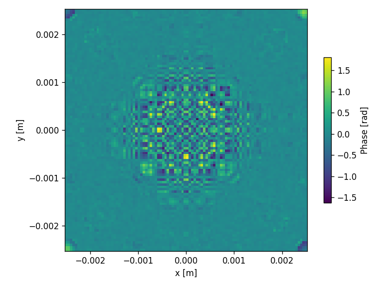
EXYZ = moe.propagate.ASM(field, screen, wavelength, pad=2500, bl=True, mode="czt" )
Exy = moe.Screen(x,y,z_box)
Exy.screen = np.reshape(EXYZ.screen[:,:, int(z_box/zmax*nzs)], np.shape(Exy.screen[:, :, :]))
Exy.screen = (np.abs(0.0 + Exy.screen)**2)**0.13
moe.plotting.plot_screen_XY(Exy, which='amplitude')
EXYZ.screen = (np.abs(0.0 + EXYZ.screen)**2)**0.13
moe.plotting.plot_screen_XY(EXYZ, z=z_box, which='amplitude')
plt.title("ASM-CZT")
Progress: [####################] 100.0%
Elapsed: 0:00:00.464959
Progress: [####################] 100.0%
Elapsed: 0:00:01.768327
ASM-CZT mode ON, with band limit.
Progress: [####################] 100.0%
Elapsed: 0:00:45.837747
[81]:
Text(0.5, 1.0, 'ASM-CZT')

[82]:
# Make circular apertures (returns also the 2D array)

wavelength = 500e-9 #m
N_box =512
M_box =4
L_box = 64e-6 #um

D_box = L_box / 8

z_box =  128e-6 #M_box / N_box / wavelength * L_box**2 * 2 #m

pixsize = L_box / N_box
x_pixel = N_box
y_pixel = N_box

aperture_width  = x_pixel*pixsize
aperture_height = y_pixel*pixsize


y_box = np.linspace(-L_box/2, L_box/2, N_box)
x_box = y_box

XX, YY =np.meshgrid(x_box, y_box)
print(np.shape(XX))


# Define Aperture
aperture = moe.generate.create_empty_aperture(-aperture_width/2, aperture_width/2, x_pixel, -aperture_height/2, aperture_height/2, y_pixel)


mask_amplitude = moe.generate.create_empty_aperture_from_aperture(aperture)

# Populate Aperture from phase mask
mask_amplitude = moe.generate.circular_aperture(aperture, radius=D_box/2-pixsize)


U_box = mask_amplitude.aperture *\
        (np.exp(1j * 2 * np.pi / wavelength * YY * np.sin(-45/ 360 * 2 * np.pi)) + \
         np.exp(1j * 2 * np.pi / wavelength * XX * np.sin(-45/ 360 * 2 * np.pi)) )


# Define Phase mask
mask_phase = moe.generate.create_empty_aperture_from_aperture(aperture)
mask_phase.aperture =  np.angle(U_box)##np.abs(U_box)*np.pi


# Plot the circular mask
moe.plotting.plot_aperture(mask_phase)

moe.plotting.plot_aperture(mask_amplitude)


# Calculates a field to use with the calculated mask

# Initialize a Field from the Aperture mask
field = moe.field.create_empty_field_from_aperture(mask_phase)

# Generate a uniform field
field = moe.field.generate_uniform_field(field, E0=1)


# Modulates the field with a given aperture that can be used either as an amplitude mask or a phase mask
field = moe.field.modulate_field(field, amplitude_mask=mask_amplitude, phase_mask=mask_phase)

# Plots the field (amplitude and phase)
moe.plotting.plot_field(field)

plt.tight_layout()
plt.show()
(512, 512)
[83]:
###Propagate field and calculate in plane YZ, using npix bins in Y
zmin = wavelength*2
zmax = 1*z_box
nzs = 2
# Creates a screen in YZ plane with [-aperture_height/2, aperture_height/2] and [zmin, zmax] and
ymin, ymax = -aperture_height/2*4, aperture_height/2*4
xmin, xmax = -aperture_height/2*4, aperture_height/2*4
#ymin, ymax = -4, 4
#xmin, xmax = ymin, ymax
x = np.linspace(xmin, xmax, x_pixel)
y = np.linspace(ymin, ymax, y_pixel)
z = np.linspace(zmin, zmax, nzs)
screen = moe.Screen(x,y,z)
# Propagate the field
EXYZ = moe.propagate.Bluestein(field, screen, wavelength)
EXYZ.screen = (np.abs(EXYZ.screen)**2)**0.13
moe.plotting.plot_screen_XY(EXYZ,z=z_box, which='amplitude')
plt.title("Bluestein")
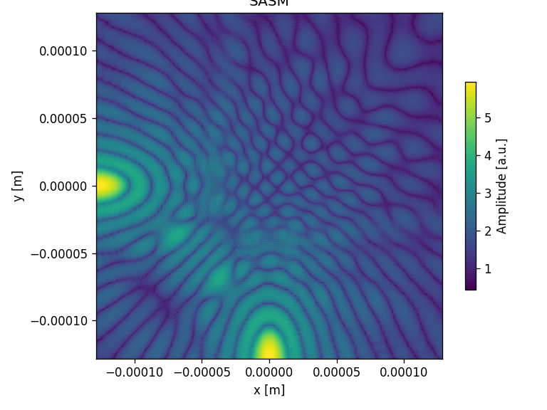
# Propagate the field with SASM
screen = moe.Screen(x,y,z)
EXYZ = moe.propagate.SASM(field, screen, wavelength, pad_factor=2, crop=True)
EXYZ.screen = (np.abs(0.0 + EXYZ.screen)**2)**0.13
moe.plotting.plot_screen_XY(EXYZ, z=z_box, which='amplitude')
plt.title("SASM")
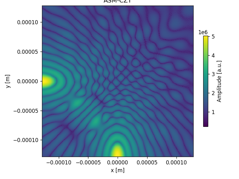
# Propagate the field with ASM-CZT
screen = moe.Screen(x,y,z)
EXYZ = moe.propagate.ASM(field, screen, wavelength, pad=2500, bl=True, mode="czt" )
EXYZ.screen = (np.abs(0.0 + EXYZ.screen)**2)**0.13
moe.plotting.plot_screen_XY(EXYZ, z=z_box, which='amplitude')
plt.title("ASM-CZT")
Progress: [####################] 100.0%
Elapsed: 0:00:00.459035
Progress: [####################] 100.0%
Elapsed: 0:00:01.823022
ASM-CZT mode ON, with band limit.
Progress: [####################] 100.0%
Elapsed: 0:00:45.977473
[83]:
Text(0.5, 1.0, 'ASM-CZT')
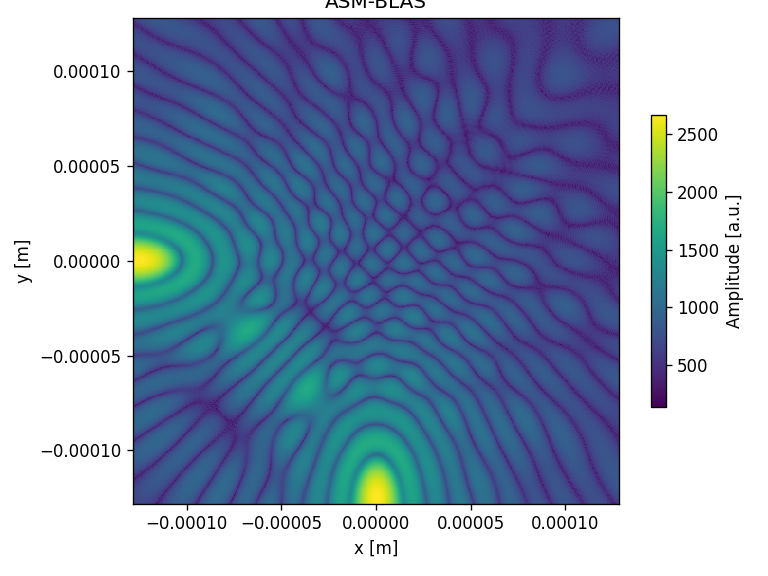
[84]:
# Propagate the field with SASM
screen = moe.Screen(x,y,z)
EXYZ = moe.propagate.ASM(field, screen, wavelength, pad=2500, bl=True, mode="BLAS" )

EXYZ.screen = (np.abs(0.0 + EXYZ.screen)**2)**0.13
moe.plotting.plot_screen_XY(EXYZ, z=z_box, which='amplitude')
plt.title("ASM-BLAS")
BLAS mode ON.
Progress: [####################] 100.0%
Elapsed: 0:02:31.163394
[84]:
Text(0.5, 1.0, 'ASM-BLAS')
[85]:
# Propagate the field with SASM
screen = moe.Screen(x,y,z)
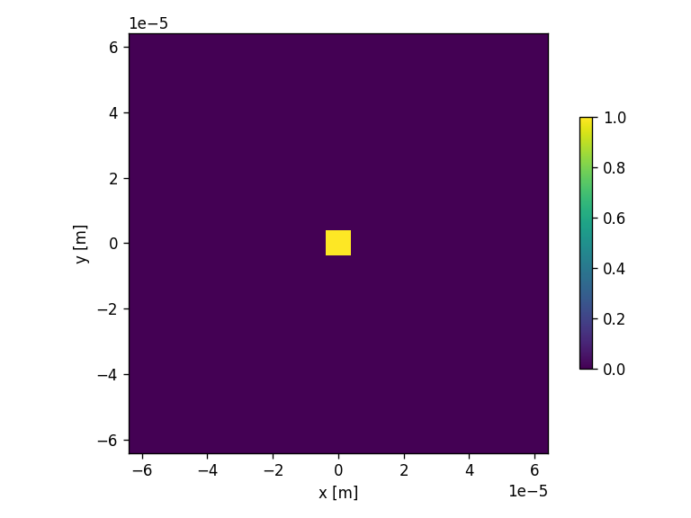
EXYZ = moe.propagate.ASM(field, screen, wavelength, pad=2500, )
EXYZ.screen = (np.abs(0.0 + EXYZ.screen)**2)**0.13
moe.plotting.plot_screen_XY(EXYZ, z=z_box, which='amplitude')
plt.title("Conventional ASM ")
Conventional ASM, without band limit.
Progress: [####################] 100.0%
Elapsed: 0:00:45.676054
[85]:
Text(0.5, 1.0, 'Conventional ASM ')
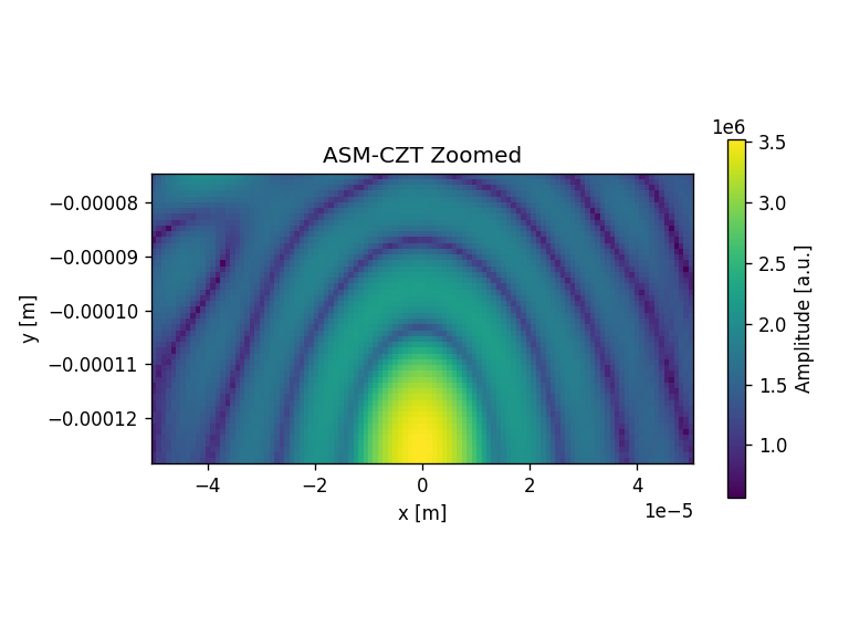
[86]:
x = np.linspace(-5e-5, 5e-5, 110)
y = np.linspace(ymin, -7.5e-5, 50)
z = np.linspace(zmin, zmax, nzs)

screen = moe.Screen(x,y,z)

# Propagate the field with ASM-CZT
EXYZ = moe.propagate.ASM(field, screen, wavelength, pad=2500,  mode="czt" )
#czt mode allows direct control on the screen - non-czt requires to provide the kxky

EXYZ.screen = (np.abs(0.0 + EXYZ.screen)**2)**0.13

moe.plotting.plot_screen_XY(EXYZ, z=z_box, which='amplitude')
plt.title("ASM-CZT Zoomed")
plt.tight_layout()
ASM-CZT mode ON, without band limit.
Progress: [####################] 100.0%
Elapsed: 0:00:42.692215
Propagation from Computer Generated Holograms
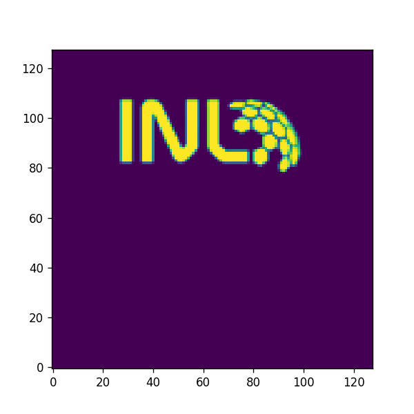
[87]:
from PIL import Image, ImageOps
file = "../5 - Holograms/target.png"

target = Image.open(file).convert("L")
target = ImageOps.flip(target)

size = 128
target = target.resize((size,size))
target = np.array(target)/255

fig = plt.figure(figsize=(5,5))
x = np.arange(0,size)
y = np.arange(0,size)
plt.pcolormesh(x,y,target)
[87]:
<matplotlib.collections.QuadMesh at 0x20c9f296d50>
[88]:
# Binary level phase mask
levels = 2

iterations = 20

levels = moe.utils.create_levels(-np.pi, np.pi, levels,)
phase_mask, errors = moe.holograms.algorithm_Gerchberg_Saxton(target, iterations=iterations, levels=levels)
phase_mask = moe.holograms.correct_mask_shift(phase_mask)

#When working in cartesian axes with apertures, attention should be given to correct the image axes to match cartesian orientation
phase_mask = np.flipud(np.rot90(phase_mask))
mask = moe.generate.create_aperture_from_array(phase_mask, pixel_size=(1*micro, 1*micro), center=True, )


# Discretize to same levels as original
mask.discretize(levels)
moe.plotting.plot_aperture(mask)
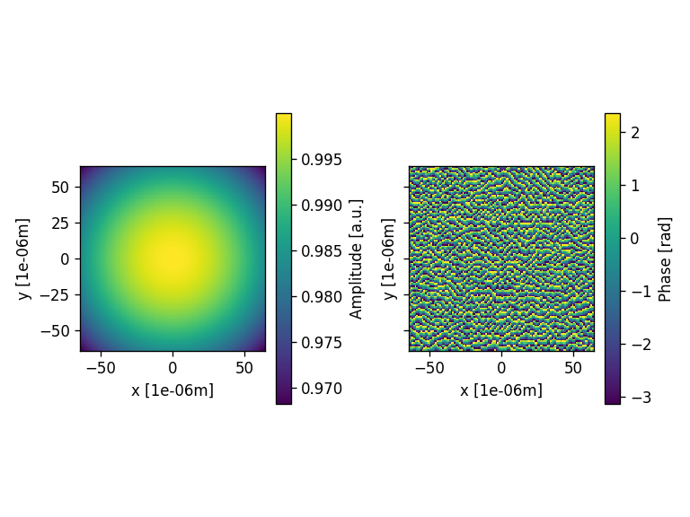
Progress: [####################] 100.0%
[Gerchberg Saxton Algorithm]
Elapsed: 0:00:00.147351

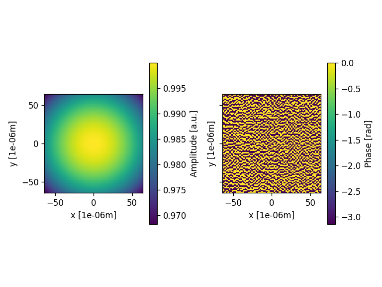
[89]:
# Create the gaussian field to propagate through the hologram

field = moe.field.create_empty_field_from_aperture(mask)
field = moe.field.generate_gaussian_field(field, E0=1, w0=500*micro)
# field = moe.field.modulate_field(field, amplitude_mask=mask, phase_mask=None)
field = moe.field.modulate_field(field, amplitude_mask=None, phase_mask=mask)

moe.plotting.plot_field(field, scale=micro)
plt.tight_layout()
Propagation of Holograms with RS integral
[90]:
# define the wavelength used in the propagation
wavelength = 532*nano
# Define the screen size and create it
screen_width = 7000*micro
screen_height = 7000*micro
x_pixel = 128
y_pixel = 128
screen_XY = moe.field.create_screen_XY(-screen_width/2, screen_width/2, x_pixel,
-screen_height/2, screen_height/2, y_pixel,
z=15000*micro)
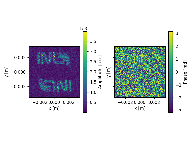
screen_XY = moe.propagate.Bluestein(field, screen_XY, wavelength)
moe.plotting.plot_screen_XY(screen_XY)
plt.tight_layout()
Progress: [####################] 100.0%
Elapsed: 0:00:00.006972
Propagation of Holograms with Bluestein
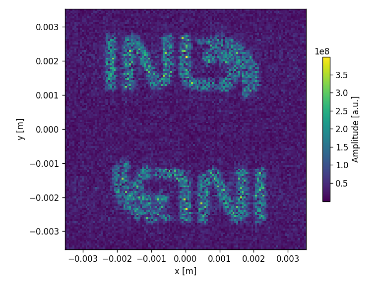
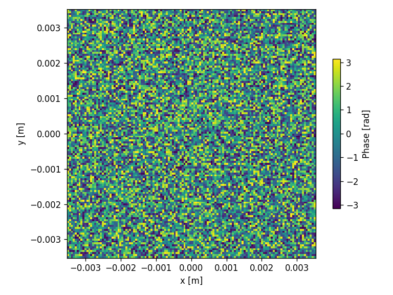
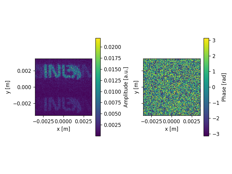
[91]:
x = np.linspace(-screen_width/2, screen_width/2, x_pixel)
y = np.linspace(-screen_height/2, screen_height/2, y_pixel,)
z = [15000*micro]

screen = moe.Screen(x,y,z)

#screen_XY3 = moe.field.create_screen_XY(-screen_width/2, screen_width/2, x_pixel,
#                                     -screen_height/2, screen_height/2, y_pixel,
#                                     z=15000*micro)

E_XY3 = moe.propagate.Bluestein(field, screen, wavelength)

moe.plotting.plot_screen_XY(E_XY3, which='amplitude')
moe.plotting.plot_screen_XY(E_XY3, which='phase')
Progress: [####################] 100.0%
Elapsed: 0:00:00.006969
Multilevel GS holograms
[92]:
# Multilevel phase hologram
levels = 8

iterations = 20

levels = moe.utils.create_levels(-np.pi, np.pi, levels,)
phase_mask, errors = moe.holograms.algorithm_Gerchberg_Saxton(target, iterations=iterations, levels=levels)

phase_mask = moe.holograms.correct_mask_shift(phase_mask)

#When working in cartesian axes with apertures, attention should be given to correct the image axes to match cartesian orientation
phase_mask = np.flipud(np.rot90(phase_mask))

mask = moe.generate.create_aperture_from_array(phase_mask, pixel_size=(1*micro, 1*micro), center=True, )


# Discretize to same levels as original
mask.discretize(levels)
moe.plotting.plot_aperture(mask)

# Create the gaussian field to propagate through the hologram
field = moe.field.create_empty_field_from_aperture(mask)
field = moe.field.generate_gaussian_field(field, E0=1, w0=500*micro)
# field = moe.field.modulate_field(field, amplitude_mask=mask, phase_mask=None)
field = moe.field.modulate_field(field, amplitude_mask=None, phase_mask=mask)


moe.plotting.plot_field(field, scale=micro)
plt.tight_layout()


# define the wavelength used in the propagation
wavelength = 532*nano

# Define the screen size and create it
screen_width = 7000*micro
screen_height = 7000*micro
x_pixel = 128
y_pixel = 128

screen_XY = moe.field.create_screen_XY(-screen_width/2, screen_width/2, x_pixel,
                                     -screen_height/2, screen_height/2, y_pixel,
                                     z=15000*micro)

screen_XY = moe.propagate.RS_integral(field, screen_XY, wavelength)

moe.plotting.plot_screen_XY(screen_XY)
plt.tight_layout()
Progress: [####################] 100.0%
[Gerchberg Saxton Algorithm]
Elapsed: 0:00:00.147352
Warning: Sampling field pixel is larger than wavelength/2!
[########################################] | 100% Completed | 53.63 s
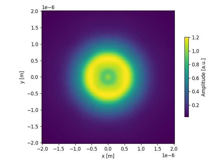
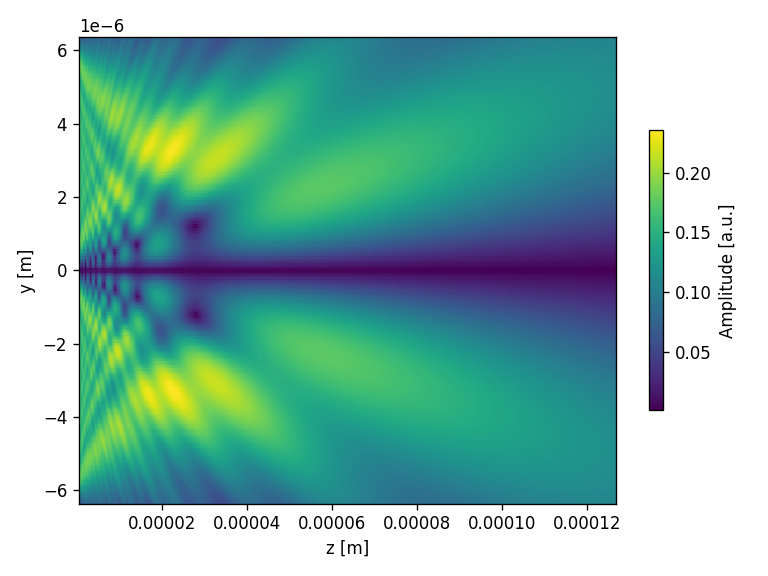
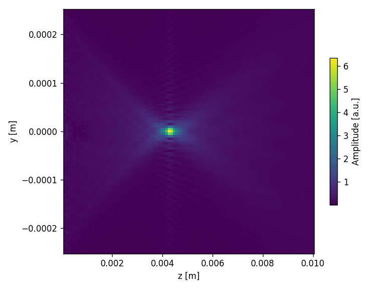
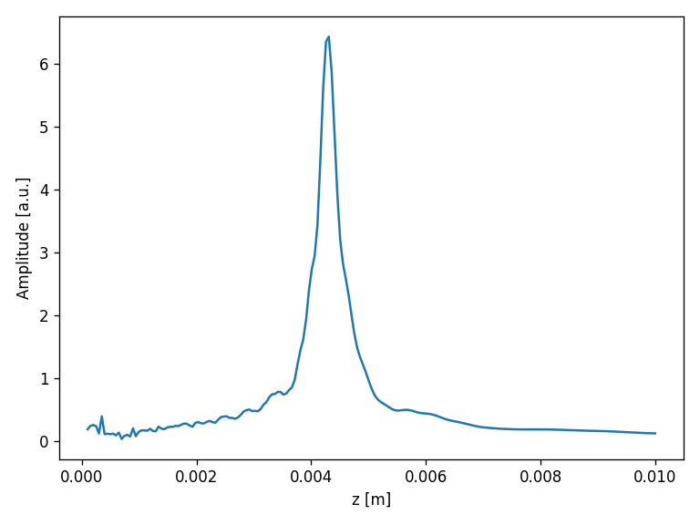
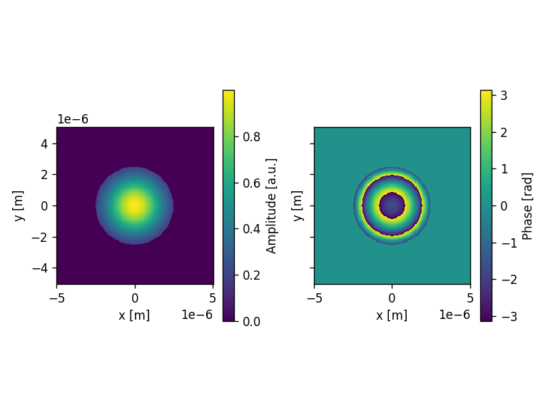
Near Field: Nanojet generation from a circular aperture illuminated by a Gaussian Beam
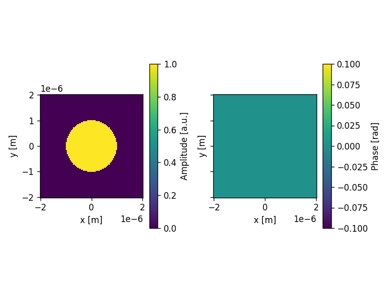
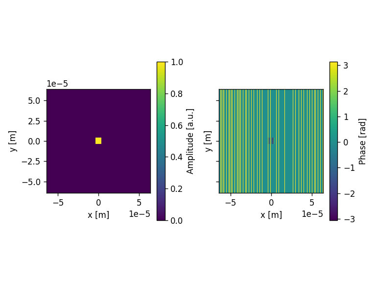
[93]:
wavelength = 500e-9 #m
zdist = 100*wavelength #m

x_pixel = 200
y_pixel = 200

radius = 2.5e-6 #m

aperture_width  = 4*radius
aperture_height = 4*radius

d = -3e-6 #displacement of the waist of the Gaussian beam

center = (-(aperture_width/x_pixel)/2, -(aperture_height/y_pixel)/2)

# Define Aperture
aperture = moe.generate.create_empty_aperture(-aperture_width/2, aperture_width/2, x_pixel, -aperture_height/2, aperture_height/2, y_pixel)

# Populate Aperture from phase mask
mask = moe.generate.circular_aperture(aperture, radius=radius, center =center )

# Define Phase mask
mask_phase = moe.generate.create_empty_aperture_from_aperture(aperture)
mask_phase.aperture = mask.aperture*np.pi

mask_phase.aperture[mask_phase.XX**2 + mask_phase.YY**2 > radius**2] = 0


# Plot the circular mask
moe.plotting.plot_aperture(mask)

moe.plotting.plot_aperture(mask_phase)


# Calculates a field to use with the calculated mask

# Initialize a Field from the Aperture mask
field = moe.field.create_empty_field_from_aperture(mask)


field = moe.field.generate_gaussian_beam(field, 0.5*wavelength, d, wavelength)


# Plots the field (amplitude and phase)
moe.plotting.plot_field(field)

plt.tight_layout()
plt.show()

# Modulates the field with a given aperture that can be used either as an amplitude mask or a phase mask
field = moe.field.modulate_field(field, amplitude_mask=mask, phase_mask=mask_phase)

field.field[mask_phase.XX**2 + mask_phase.YY**2 > radius**2] = 0

# Plots the field (amplitude and phase)
moe.plotting.plot_field(field)

plt.tight_layout()
plt.show()

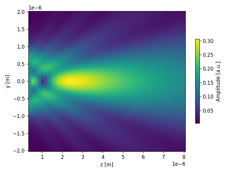
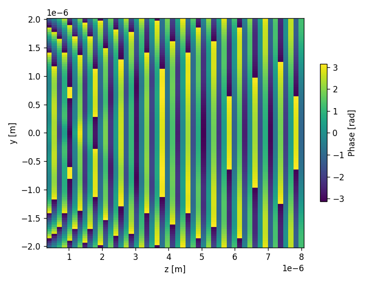
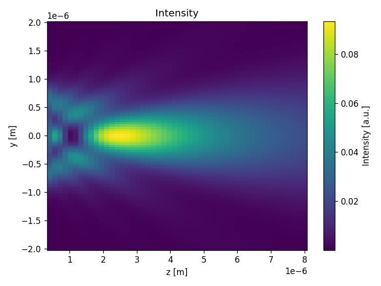
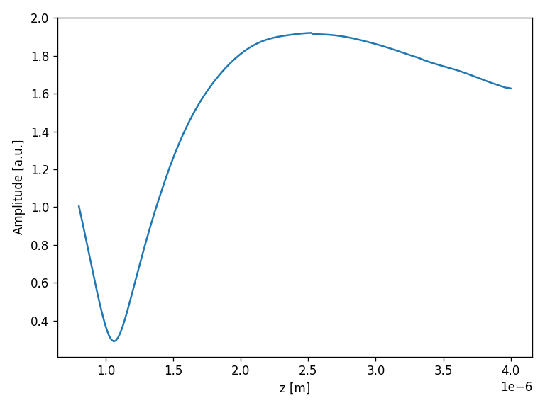
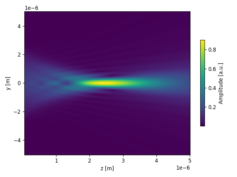
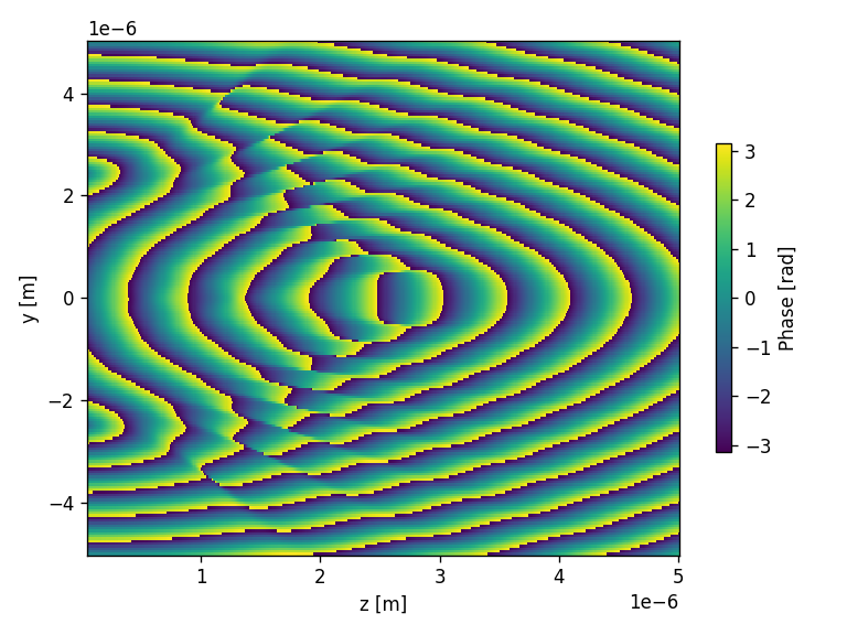
Propagate with RS
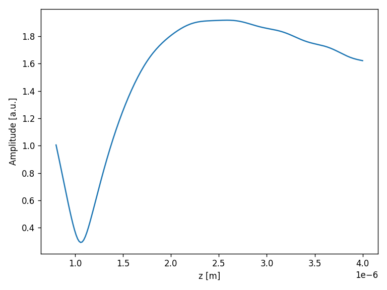
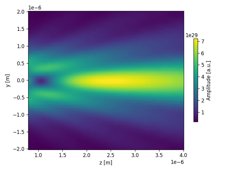
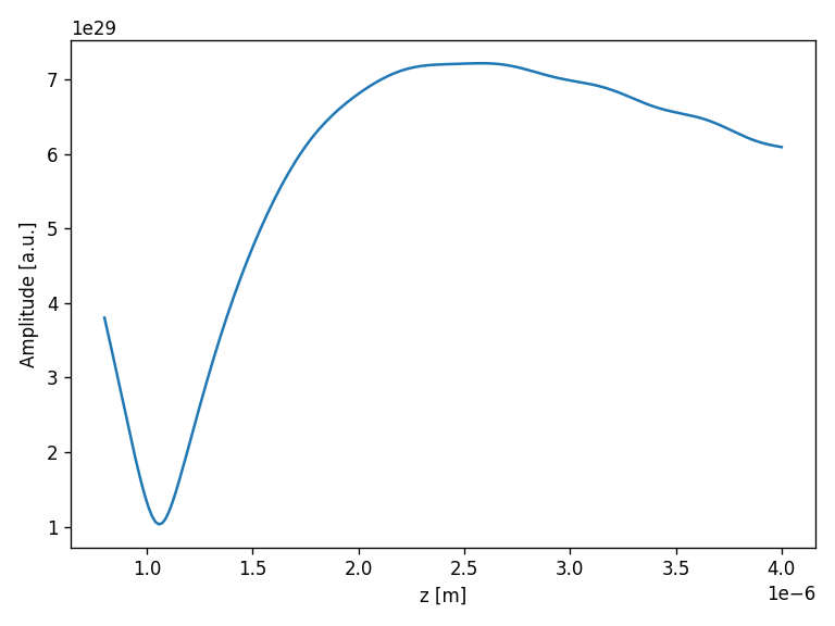
[94]:
zmin = 0.1*wavelength
zmax = 5e-6
nzs = 500

# Creates a screen in YZ plane with [-aperture_height/2, aperture_height/2] and [zmin, zmax]
screen_YZ1 = moe.field.create_screen_YZ(-aperture_height/2, aperture_height/2, y_pixel,
                                        zmin, zmax, nzs,
                                        x=0)


# Propagate the field
E_YZ = moe.propagate.RS_integral(field, screen_YZ1,  wavelength, simp2d=True)

#Plot the amplitude of the propagated field in yz screen
moe.plotting.plot_screen_YZ(E_YZ, which='amplitude')
plt.show()

#Plot the phase of the propagated field in yz screen
moe.plotting.plot_screen_YZ(E_YZ, which='phase')
plt.show()
[########################################] | 100% Completed | 273.33 s
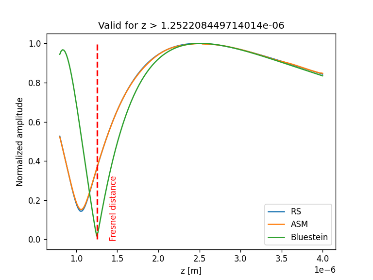
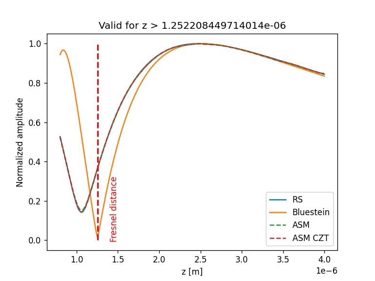
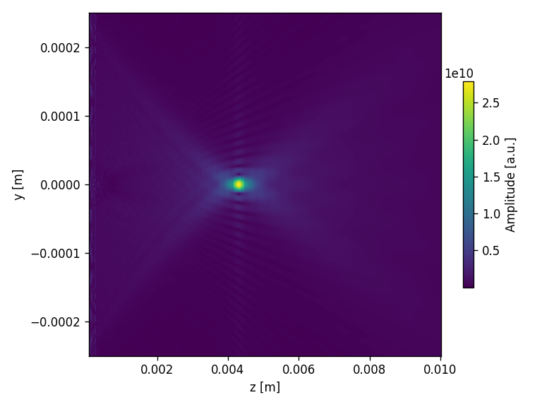
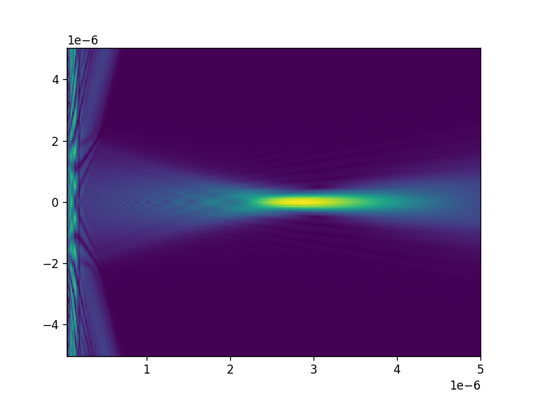
Propagate with Bluestein
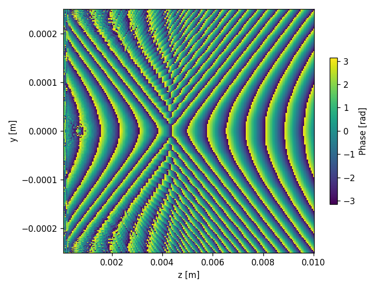
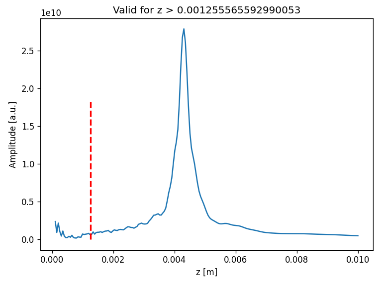
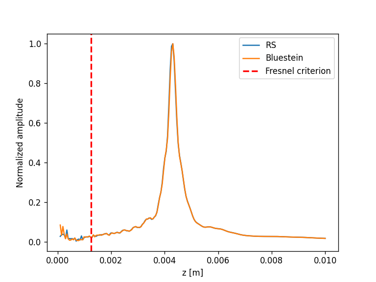
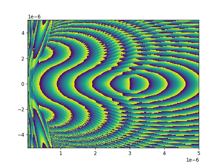
[95]:
#Propagate with Bluestein

screen_YZ1 = moe.field.create_screen_YZ(-aperture_height/2, aperture_height/2, y_pixel,
                                        zmin, zmax, nzs,
                                        x=0)

E_XY3 = moe.propagate.Bluestein(field, screen_YZ1,  wavelength)
C:\Users\jcunha377\Desktop\pyMOE-main-v2.0\notebooks\6 - Propagation\../..\pyMOE\propagate.py:353: RuntimeWarning: divide by zero encountered in scalar divide
  w = np.exp(-1j * 2 * np.pi / ((mout * fs) /((f22 - f11) )))
Progress: [####################] 100.0%
Elapsed: 0:00:02.961167
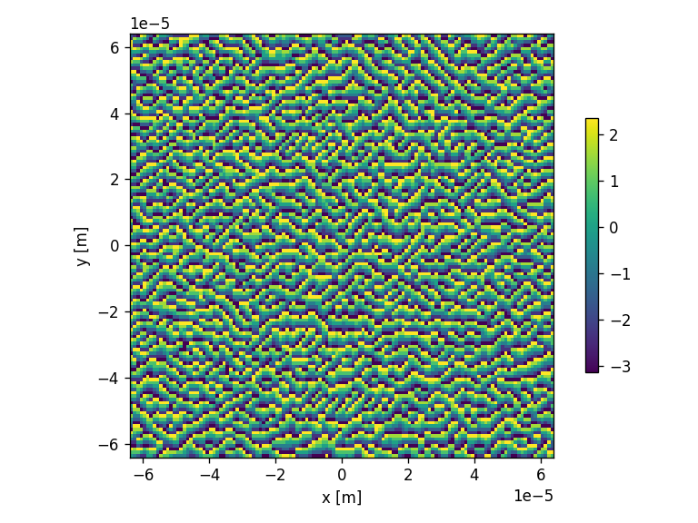
[96]:
#moe.plotting.plot_screen_XY(E_XY3.screen[:,0,:], which='amplitude')
#moe.plotting.plot_screen_XY(E_XY3, which='phase')
[97]:
plt.figure()
plt.pcolormesh(E_XY3.z,E_XY3.y,(np.abs(E_XY3.screen[0,:,:]) ))
plt.figure()
plt.pcolormesh(E_XY3.z,E_XY3.y,np.angle(E_XY3.screen[0,:,:]) )
[97]:
<matplotlib.collections.QuadMesh at 0x20c9eee0810>
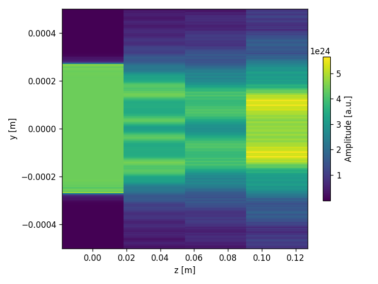
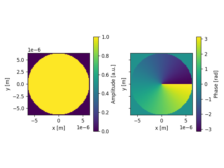
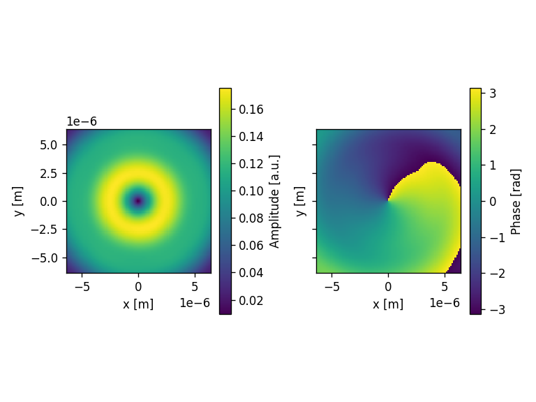
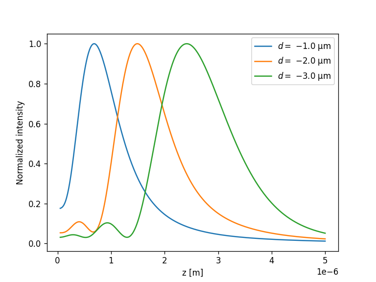
Propagate the field from a circular aperture illuminated by a tightly focused Gaussian Beam
[98]:
#### Propagate the field from a circular aperture illuminated by a tightly focused Gaussian Beam


wavelength = 500e-9 #m
zdist = 100*wavelength #m
k = 2*np.pi/(wavelength)

zmin = 0.1*wavelength
zmax = 5e-6
nzs = 500


x_pixel = 512
y_pixel = 512

radius = 2.5e-6 #m

aperture_width  = 4*radius
aperture_height = 4*radius

center = (0, 0)

vals = np.zeros((3,nzs))

fig = plt.figure()

for ids, d in enumerate(np.array([-1e-6, -2e-6, -3e-6 ])):
    # Define Aperture
    aperture = moe.generate.create_empty_aperture(-aperture_width/2, aperture_width/2, x_pixel, -aperture_height/2, aperture_height/2, y_pixel)

    # Populate Aperture from phase mask
    mask = moe.generate.circular_aperture(aperture, radius=radius)

    # Define Phase mask
    mask_phase = moe.generate.create_empty_aperture_from_aperture(aperture)
    mask_phase.aperture = mask.aperture*np.pi

    # Initialize a Field from the Aperture mask
    field = moe.field.create_empty_field_from_aperture(mask)

    field_gauss = moe.field.generate_gaussian_beam(field, 0.5*wavelength, d, wavelength)

    # Modulates the field with a given aperture that can be used either as an amplitude mask or a phase mask
    field = moe.field.modulate_field(field_gauss, amplitude_mask=mask, phase_mask=mask_phase)

    field.field[mask_phase.XX**2 + mask_phase.YY**2 > radius**2] = 0

    screen_ZZ = moe.field.create_screen_ZZ(zmin, zmax, nzs)
    E_ZZ = moe.propagate.RS_integral(field, screen_ZZ, wavelength, parallel_computing=True)

    vals[ids] = np.abs(E_ZZ.amplitude[0,0,:])**2/np.max(np.abs(E_ZZ.amplitude[0,0,:])**2)

    plt.plot(np.linspace(zmin,zmax,nzs), np.abs(E_ZZ.amplitude[0,0,:])**2/np.max(np.abs(E_ZZ.amplitude[0,0,:])**2),\
            label="$d = $ $"+str(d*1e6)+"$ $\mathrm{\mu m}$" )

###Print the distances for the two criteria
print(moe.propagate.Fresnel_criterion(wavelength, radius))
print(moe.propagate.Fraunhofer_criterion(wavelength, radius))

plt.legend()
plt.xlabel("z [m]")
plt.ylabel("Normalized intensity")
plt.show()
[########################################] | 100% Completed | 14.19 s
[########################################] | 100% Completed | 13.98 s
[########################################] | 100% Completed | 14.06 s
3.944209461627281e-06
3.926990816987243e-05
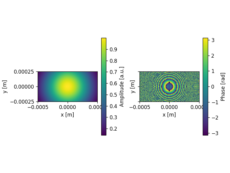
Evaluation of Oblique Incidence fields
[99]:
###let's use previous example to demonstrate how to handle oblique incidence

wavelength = 500e-9 #m
zdist = 100*wavelength #m

x_pixel = 100
y_pixel = 100

radius = 2.5e-6 #m

aperture_width  = 4*radius
aperture_height = 4*radius

d = -3e-6 #displacement of the waist of the Gaussian beam

center = (-(aperture_width/x_pixel)/2, -(aperture_height/y_pixel)/2)

# Define Aperture
aperture = moe.generate.create_empty_aperture(-aperture_width/2, aperture_width/2, x_pixel, -aperture_height/2, aperture_height/2, y_pixel)

# Populate Aperture from phase mask
mask = moe.generate.circular_aperture(aperture, radius=1*radius, center =center )

# Define Phase mask
mask_phase = moe.generate.create_empty_aperture_from_aperture(aperture)
mask_phase.aperture = mask.aperture*np.pi

mask_phase.aperture[mask_phase.XX**2 + mask_phase.YY**2 > (1*radius)**2] = 0


# Plot the circular mask
moe.plotting.plot_aperture(mask)

moe.plotting.plot_aperture(mask_phase)


# Calculates a field to use with the calculated mask

# Initialize a Field from the Aperture mask
field = moe.field.create_empty_field_from_aperture(mask)


field = moe.field.generate_gaussian_beam(field, 0.5*wavelength, d, wavelength)


#Oblique incidence angles
thetax = 0
thetay = np.pi/4
moe.plotting.plot_field(field)

#calculate the oblique field at the aperture plane
field = moe.field.oblique(field, wavelength, thetax, thetay)


# Plots the field (amplitude and phase)
moe.plotting.plot_field(field)

plt.tight_layout()
plt.show()

# Modulates the field with a given aperture that can be used either as an amplitude mask or a phase mask
field = moe.field.modulate_field(field, amplitude_mask=mask, phase_mask=mask_phase)

field.field[mask_phase.XX**2 + mask_phase.YY**2 > (1*radius)**2] = 0

# Plots the field (amplitude and phase)
moe.plotting.plot_field(field)

plt.tight_layout()
plt.show()

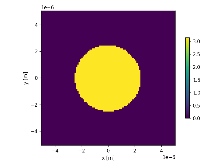


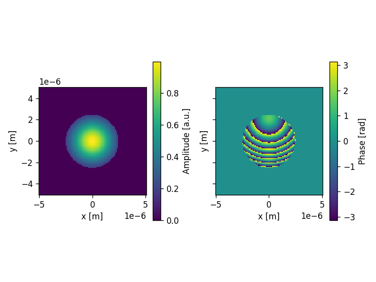
Propagation with RS
[100]:
##Propagate field in plane XY at z_distance

z_distance = d

# Creates XY screen
screen_XY = moe.field.create_screen_XY(-aperture_width/2, aperture_width/2, x_pixel,
                                       -aperture_height/2, aperture_height/2, y_pixel,
                                        z=z_distance)

# Propagate the field
E_XY = moe.propagate.RS_integral(field, screen_XY, wavelength, simp2d=True)

moe.plotting.plot_screen_XY(E_XY, which='amplitude')
plt.title("Propagated field to z = "+str(z_distance)+" m")

plt.tight_layout()
plt.show()
[########################################] | 100% Completed | 31.05 s
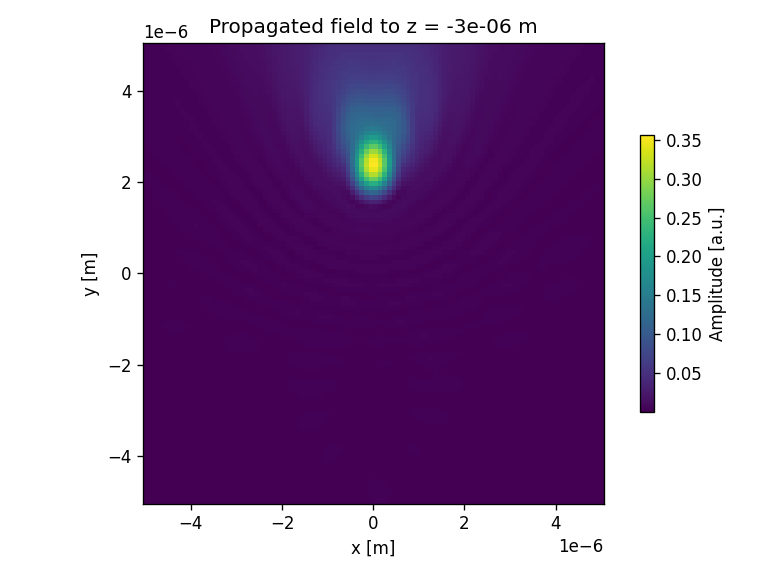
Propagation with Bluestein XY YZ
[101]:
#Simple oblique propagate in YZ

wavelength = 500e-9 #m
zdist = 100*wavelength #m

x_pixel = 200
y_pixel = 200

radius = 2.5e-6 #m

aperture_width  = 4*radius
aperture_height = 4*radius

d = -3e-6 #displacement of the waist of the Gaussian beam

center = (-(aperture_width/x_pixel)/2, -(aperture_height/y_pixel)/2)

# Define Aperture
aperture = moe.generate.create_empty_aperture(-aperture_width/2, aperture_width/2, x_pixel, -aperture_height/2, aperture_height/2, y_pixel)


# Calculates a field to use with the calculated mask

# Initialize a Field from the Aperture mask
field = moe.field.create_empty_field_from_aperture(aperture)


field = moe.field.generate_gaussian_beam(field, 0.5*wavelength, d, wavelength)

moe.plotting.plot_field(field)

field = moe.field.oblique(field, wavelength, 0, np.pi/4)

# Plots the field (amplitude and phase)
moe.plotting.plot_field(field)

plt.tight_layout()
plt.show()

# Modulates the field with a given aperture that can be used either as an amplitude mask or a phase mask
field = moe.field.modulate_field(field, amplitude_mask=None, phase_mask=None)

# Plots the field (amplitude and phase)
moe.plotting.plot_field(field)

plt.tight_layout()
plt.show()


###Propagate field and calculate in plane YZ, using npix bins in Y
zmin = 0.1*wavelength
zmax = 5e-6
nzs = 100

# Creates a screen in YZ plane with [-aperture_height/2, aperture_height/2] and [zmin, zmax] and
ymin, ymax = -aperture_height/2, aperture_height/2
xmin, xmax = -aperture_height/2, aperture_height/2

x = np.linspace(xmin, xmax, x_pixel)
y = np.linspace(ymin, ymax, y_pixel)
z = np.linspace(zmin, zmax, nzs)

screen = moe.Screen(x,y,z)

# Propagate the field
EXYZ = moe.propagate.Bluestein(field, screen, wavelength)


moe.plotting.plot_screen_YZ(EXYZ, which='amplitude')
moe.plotting.plot_screen_XZ(EXYZ, which='amplitude')

limitx = moe.propagate.Fresnel_criterion(wavelength,radius)
#plt.vlines(limitx, -radius, radius, colors='red', linestyles='dashed', lw=2)

plt.title("Valid for z > "+str(limitx))

plt.show()


moe.plotting.plot_screen_XY(EXYZ, z=2.5e-6, which='amplitude')
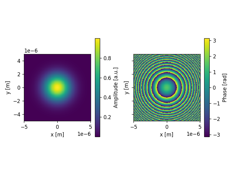

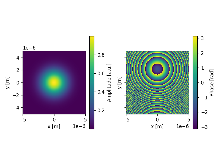
Progress: [####################] 100.0%
Elapsed: 0:00:02.607635
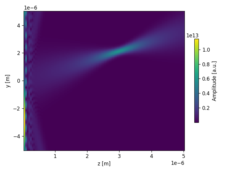
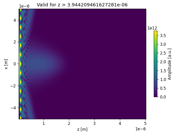
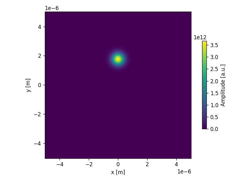
[102]:
wavelength = 500e-9 #m
zdist = 100*wavelength #m

x_pixel = 200
y_pixel = 200

radius = 2.5e-6 #m

aperture_width  = 4*radius
aperture_height = 4*radius

d = -3e-6 #displacement of the waist of the Gaussian beam

center = (-(aperture_width/x_pixel)/2, -(aperture_height/y_pixel)/2)

# Define Aperture
aperture = moe.generate.create_empty_aperture(-aperture_width/2, aperture_width/2, x_pixel, -aperture_height/2, aperture_height/2, y_pixel)


# Calculates a field to use with the calculated mask

# Initialize a Field from the Aperture mask
field = moe.field.create_empty_field_from_aperture(aperture)


field = moe.field.generate_gaussian_beam(field, 0.5*wavelength, d, wavelength)

moe.plotting.plot_field(field)

field = moe.field.oblique(field, wavelength, np.pi/4, np.pi/4)

# Plots the field (amplitude and phase)
moe.plotting.plot_field(field)

plt.tight_layout()
plt.show()

# Modulates the field with a given aperture that can be used either as an amplitude mask or a phase mask
field = moe.field.modulate_field(field, amplitude_mask=None, phase_mask=None)

# Plots the field (amplitude and phase)
moe.plotting.plot_field(field)

plt.tight_layout()
plt.show()


###Propagate field and calculate in plane YZ, using npix bins in Y
zmin = wavelength*4
zmax = 5e-6
nzs = 100

# Creates a screen in YZ plane with [-aperture_height/2, aperture_height/2] and [zmin, zmax] and
ymin, ymax = -aperture_height/2, aperture_height/2
xmin, xmax = -aperture_height/2, aperture_height/2

x = np.linspace(xmin, xmax, x_pixel)
y = np.linspace(ymin, ymax, y_pixel)
z = np.linspace(zmin, zmax, nzs)

screen = moe.Screen(x,y,z)

# Propagate the field
EXYZ = moe.propagate.Bluestein(field, screen, wavelength)


moe.plotting.plot_screen_YZ(EXYZ, x=0, which='amplitude')
moe.plotting.plot_screen_YZ(EXYZ, x=2.5e-6, which='amplitude')

limitx = moe.propagate.Fresnel_criterion(wavelength,radius)
#plt.vlines(limitx, -radius, radius, colors='red', linestyles='dashed', lw=2)

plt.title("Valid for z > "+str(limitx))

plt.show()

Exy = moe.Screen(x,y,2.5e-6)
Exy.screen = np.reshape(EXYZ.screen[:,:, int(2.5e-6/zmax*nzs)], np.shape(Exy.screen[:, :, :]))


moe.plotting.plot_screen_XY(Exy, which='amplitude')


Progress: [####################] 100.0%
Elapsed: 0:00:02.525518
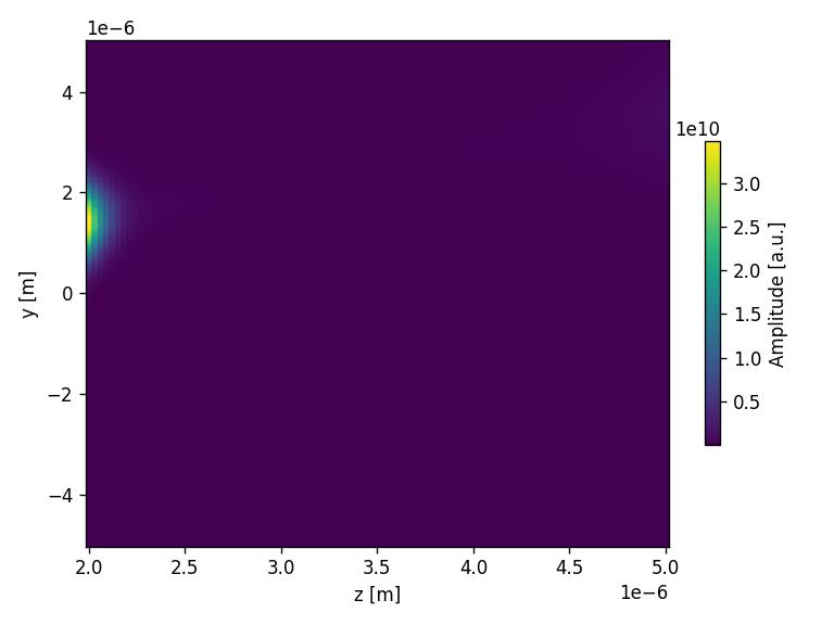
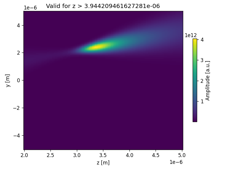
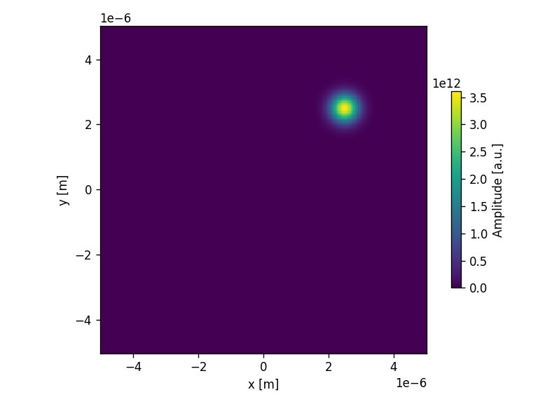
Propagation through two lenses
Manually propagate through two sequential apertures
[103]:
###Import two surfaces - doublet
import numpy as np

a1_phase = np.genfromtxt("asph1_phase.csv", delimiter=',')
a1_inten = np.genfromtxt("asph1_inten.csv", delimiter=',')

a2_phase = np.genfromtxt("asph2_phase.csv", delimiter=',')
a2_inten = np.genfromtxt("asph2_inten.csv", delimiter=',')

a1_phase.shape
[103]:
(400, 400)
[104]:
#number of pixels
x_pixel, y_pixel = a1_phase.shape

#size of the rectangular mask
aperture_width  = 0.2e-3 #m
aperture_height = 0.2e-3

pixsize = 0.5e-6 #m

wavelength = 700e-9 #m

dist1 = 0.1e-3
dist2 = 0.4e-3

zmin1 = wavelength
zmax1 = dist1
nzs = 200

zmin2 = 0.1*wavelength
zmax2 = 1.2* dist2
nzs = 200


radius = aperture_width/2
[105]:
asph1_mask_phase = moe.generate.create_empty_aperture(-aperture_width/2, aperture_width/2, x_pixel, -aperture_height/2, aperture_height/2, y_pixel)
asph1_mask_phase.aperture = a1_phase

asph1_mask_inten = moe.generate.create_empty_aperture_from_aperture(asph1_mask_phase)
asph1_mask_inten.aperture = a1_inten

# Initialize a Field from the Aperture mask
field1 = moe.field.create_empty_field_from_aperture(asph1_mask_phase)

# Generate a uniform field
field1 = moe.field.generate_uniform_field(field1, E0=1)

# Modulates the field with a given aperture that can be used either as an amplitude mask or a phase mask
field1 = moe.field.modulate_field(field1, amplitude_mask = asph1_mask_inten, phase_mask=asph1_mask_phase)

# Plots the field (amplitude and phase)
moe.plotting.plot_field(field1)

plt.tight_layout()
plt.show()


asph2_mask_phase = moe.generate.create_empty_aperture(-aperture_width/2, aperture_width/2, x_pixel, -aperture_height/2, aperture_height/2, y_pixel)
asph2_mask_phase.aperture = a2_phase

asph2_mask_inten = moe.generate.create_empty_aperture_from_aperture(asph2_mask_phase)
asph2_mask_inten.aperture = a2_inten

# Initialize a Field from the Aperture mask
field2 = moe.field.create_empty_field_from_aperture(asph2_mask_phase)

# Generate a uniform field
field2 = moe.field.generate_uniform_field(field2, E0=1)

# Modulates the field with a given aperture that can be used either as an amplitude mask or a phase mask
field2 = moe.field.modulate_field(field2, amplitude_mask = asph2_mask_inten, phase_mask=asph2_mask_phase)

# Plots the field (amplitude and phase)
moe.plotting.plot_field(field2)

plt.tight_layout()
plt.show()
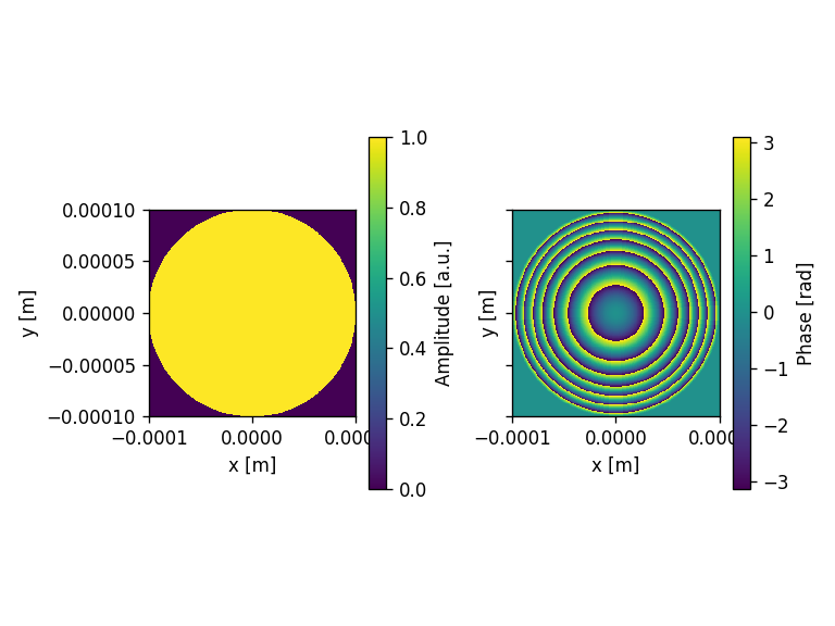
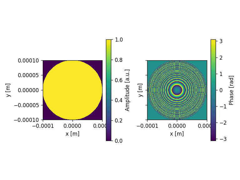
[106]:
x1 = asph1_mask_phase.x
y1 = asph1_mask_phase.y
z1 = np.linspace(zmin1, zmax1, nzs)

screen1 = moe.Screen(x1,y1,z1)

x2 = asph2_mask_phase.x
y2 = asph2_mask_phase.y
z2 = np.linspace(zmin2, zmax2, nzs)

screen2 = moe.Screen(x2,y2,z2)
[107]:
# Propagate the field
EXYZ1 = moe.propagate.Bluestein(field1, screen1, wavelength)
Progress: [####################] 100.0%
Elapsed: 0:00:30.392207
[108]:
Eyz1 = moe.Screen(0,y1,z1)
Eyz1.screen = np.reshape(np.abs(EXYZ1.screen[:,int(y_pixel/2),:]), np.shape(Eyz1.screen[:, :, :]))

moe.plotting.plot_screen_YZ(Eyz1, which='amplitude')

limitx = moe.propagate.Fresnel_criterion(wavelength,aperture_width)
#plt.vlines(limitx, -aperture_width/2, aperture_width/2, colors='red', linestyles='dashed', lw=2)
#plt.annotate("Fresnel distance", (limitx-limitx*0.1,-0.002), rotation="vertical", color="Red")

plt.title("|$E^2$| \n Valid for z > "+str(limitx))
plt.tight_layout()
plt.show()


Exy1 = moe.Screen(x1,y1,0)

fig = plt.figure(figsize=(5,4.5))
plt.pcolormesh(x1,y1, np.abs(EXYZ1.screen[:,:, -1]), shading='gouraud')
plt.title("Amplitude |$E$|")

plt.xlabel("x [m]")
plt.ylabel("y [m]")
plt.tight_layout()
plt.axis('equal')
plt.tight_layout()
plt.show()
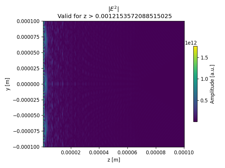
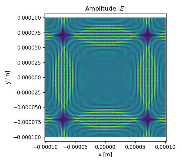
[109]:
field2.field = EXYZ1.screen[:,:, -1]/np.max(EXYZ1.screen[:,:, -1])

# Modulates the field with a given aperture that can be used either as an amplitude mask or a phase mask
field2 = moe.field.modulate_field(field2, amplitude_mask = asph2_mask_inten, phase_mask=asph2_mask_phase)

# Plots the field (amplitude and phase)
moe.plotting.plot_field(field2)

plt.tight_layout()
plt.show()
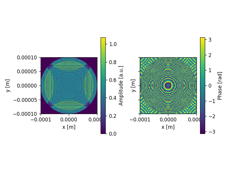
[110]:
# Propagate the field
EXYZ2 = moe.propagate.Bluestein(field2, screen2, wavelength)
Progress: [####################] 100.0%
Elapsed: 0:00:30.251306
[111]:
Eyz2 = moe.Screen(0,y2,z2)
Eyz2.screen = np.reshape(np.abs(EXYZ2.screen[:,int(y_pixel/2), :]), np.shape(Eyz2.screen[:, :, :]))

moe.plotting.plot_screen_YZ(Eyz2, which='amplitude')

limitx = moe.propagate.Fresnel_criterion(wavelength,aperture_width/2)
plt.vlines(limitx, -aperture_width/2, aperture_width/2, colors='red', linestyles='dashed', lw=2)
#plt.annotate("Fresnel distance", (limitx-limitx*0.1,-0.002), rotation="vertical", color="Red")

plt.title("|$E^2$| \n Valid for z > "+str(limitx))
plt.tight_layout()
plt.show()


Exy2 = moe.Screen(x2,y2,0)

fig = plt.figure(figsize=(5,4.5))
plt.pcolormesh(x2,y2, np.abs(EXYZ2.screen[:,:, int(0.3e-3/zmax2*nzs)]), shading='gouraud')
plt.title("Amplitude |$E$|")

plt.xlabel("x [m]")
plt.ylabel("y [m]")
plt.tight_layout()
plt.axis('equal')
plt.tight_layout()
plt.show()
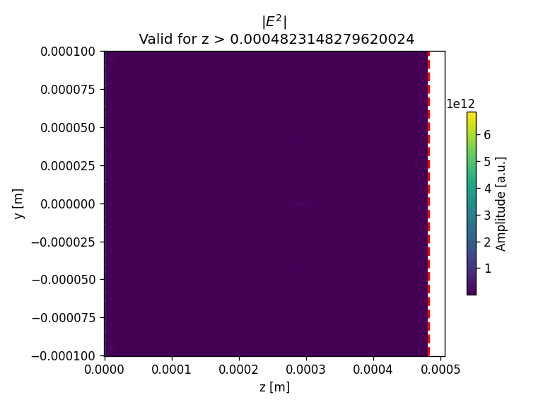
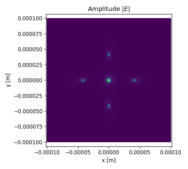
[112]:
np.abs(EXYZ1.screen[:,int(y_pixel/2), :]).shape, EXYZ1.screen[:,:,:].shape
array_screens = np.array([EXYZ1.screen, EXYZ2.screen])
[113]:
Exy_Bluestein_stack = np.dstack(array_screens)
print(Exy_Bluestein_stack.shape)
(400, 400, 400)
[114]:
Exy_Bluestein_all =  np.abs(Exy_Bluestein_stack[:,int(y_pixel/2), :])
print(Exy_Bluestein_all.shape)

zall = np.hstack((Eyz1.z, Eyz2.z+np.max(Eyz1.z)) )
yall = Eyz1.y

print(yall.shape, zall.shape)

fig = plt.figure(figsize=(6,4))
plt.pcolormesh(zall, yall, Exy_Bluestein_all, vmax=1e11)
plt.xlabel("z [m]")
plt.ylabel("y [m]")
plt.tight_layout()
plt.colorbar()

plt.vlines([zmin1+wavelength, zmin2+np.max(Eyz1.z)], -aperture_width/2, aperture_width/2, colors='white', linestyles='dashed', lw=2, \
           label="Lenses Surfaces Positions")
#plt.annotate("Fresnel distance", (limitx-limitx*0.1,-0.002), rotation="vertical", color="Red")

#plt.annotate("Fresnel distance", (limitx-limitx*0.1,-0.002), rotation="vertical", color="Red")

plt.title("Sequential Bluestein propagation through system of lenses")
plt.legend()

plt.savefig("multilens_all_bluestein.png", dpi=600)
(400, 400)
(400,) (400,)
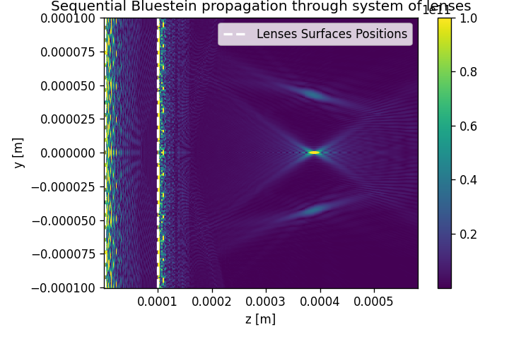
[115]:
Exy_Bluestein_all = np.hstack((np.abs(EXYZ1.screen[:,int(y_pixel/2), :])/np.max(np.abs(EXYZ1.screen[:,int(y_pixel/2), :])),\
                               np.abs(EXYZ2.screen[:,int(y_pixel/2), :])/np.max(np.abs(EXYZ2.screen[:,int(y_pixel/2), :]))))
print(Exy_Bluestein_all.shape)

zall = np.hstack((Eyz1.z, Eyz2.z+np.max(Eyz1.z) ))
yall = Eyz1.y

print(yall.shape, zall.shape)

fig = plt.figure(figsize=(7,4))
plt.pcolormesh(zall, yall, np.log(Exy_Bluestein_all) )
plt.xlabel("z [m]")
plt.ylabel("y [m]")
plt.tight_layout()

plt.vlines([zmin1+wavelength, zmin2+np.max(Eyz1.z)], -aperture_width/2, aperture_width/2, colors='white', linestyles='dashed', lw=2, \
           label="Lenses Surfaces Positions")
#plt.annotate("Fresnel distance", (limitx-limitx*0.1,-0.002), rotation="vertical", color="Red")

plt.title("Sequential Bluestein propagation through system of lenses")
plt.legend()
plt.colorbar()

plt.savefig("multilens_all_bluestein-log.png", dpi=600)
(400, 400)
(400,) (400,)
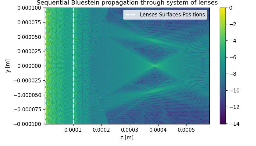
[116]:
# Propagate the field
EXYZ1 = moe.propagate.ASM(field1, screen1, wavelength, pad=500, bl=True)
Conventional ASM, with band limit.
Progress: [####################] 100.0%
Elapsed: 0:04:33.053292
[117]:
Eyz1 = moe.Screen(0,y1,z1)
Eyz1.screen = np.reshape(np.abs(EXYZ1.screen[:,int(y_pixel/2),:]), np.shape(Eyz1.screen[:, :, :]))

moe.plotting.plot_screen_YZ(Eyz1, which='amplitude')

limitx = moe.propagate.Fresnel_criterion(wavelength,aperture_width)
#plt.vlines(limitx, -aperture_width/2, aperture_width/2, colors='red', linestyles='dashed', lw=2)
#plt.annotate("Fresnel distance", (limitx-limitx*0.1,-0.002), rotation="vertical", color="Red")

plt.title("|$E^2$| \n Valid for z > "+str(limitx))
plt.tight_layout()
plt.show()


Exy1 = moe.Screen(x1,y1,0)

fig = plt.figure(figsize=(5,4.5))
plt.pcolormesh(x1,y1, np.abs(EXYZ1.screen[:,:, -1]), shading='gouraud')
plt.title("Amplitude |$E$|")

plt.xlabel("x [m]")
plt.ylabel("y [m]")
plt.tight_layout()
plt.axis('equal')
plt.tight_layout()
plt.show()
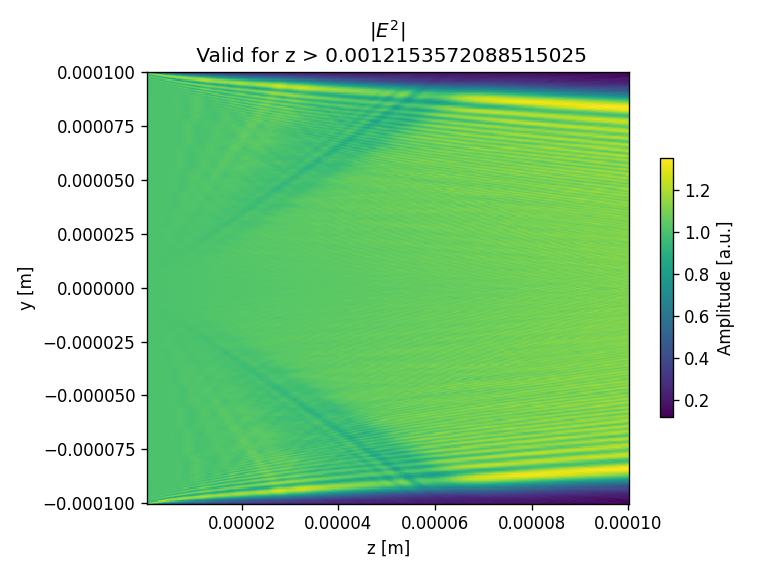
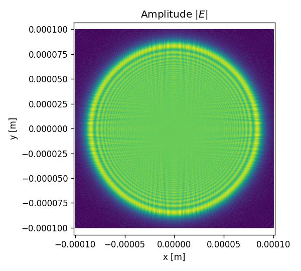
[118]:
field2.field = EXYZ1.screen[:,:, -1]/np.max(EXYZ1.screen[:,:, -1])

# Modulates the field with a given aperture that can be used either as an amplitude mask or a phase mask
field2 = moe.field.modulate_field(field2, amplitude_mask = asph2_mask_inten, phase_mask=asph2_mask_phase)

# Plots the field (amplitude and phase)
moe.plotting.plot_field(field2)

plt.tight_layout()
plt.show()
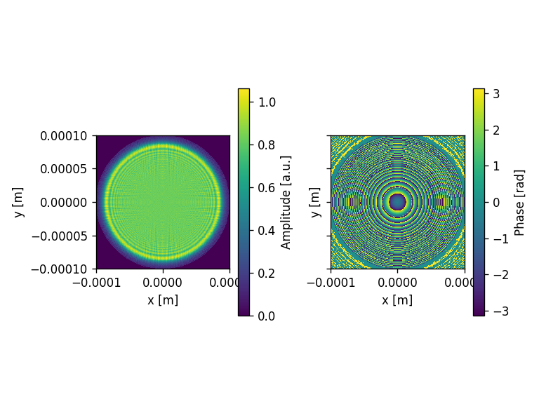
[119]:
# Propagate the field
EXYZ2 = moe.propagate.Bluestein(field2, screen2, wavelength)
Progress: [####################] 100.0%
Elapsed: 0:00:30.189371
[120]:
Eyz2 = moe.Screen(0,y2,z2)
Eyz2.screen = np.reshape(np.abs(EXYZ2.screen[:,int(y_pixel/2), :]), np.shape(Eyz2.screen[:, :, :]))

moe.plotting.plot_screen_YZ(Eyz2, which='amplitude')

limitx = moe.propagate.Fresnel_criterion(wavelength,aperture_width/2)
plt.vlines(limitx, -aperture_width/2, aperture_width/2, colors='red', linestyles='dashed', lw=2)
#plt.annotate("Fresnel distance", (limitx-limitx*0.1,-0.002), rotation="vertical", color="Red")

plt.title("|$E^2$| \n Valid for z > "+str(limitx))
plt.tight_layout()
plt.show()


Exy2 = moe.Screen(x2,y2,0)

fig = plt.figure(figsize=(5,4.5))
plt.pcolormesh(x2,y2, np.abs(EXYZ2.screen[:,:, int(0.3e-3/zmax2*nzs)]), shading='gouraud')
plt.title("Amplitude |$E$|")

plt.xlabel("x [m]")
plt.ylabel("y [m]")
plt.tight_layout()
plt.axis('equal')
plt.tight_layout()
plt.show()
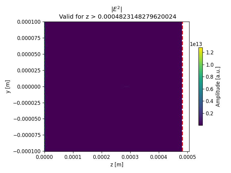
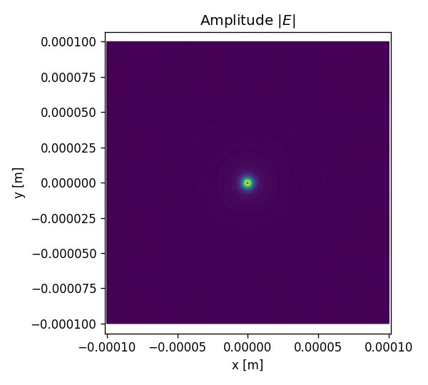
[121]:
np.abs(EXYZ1.screen[:,int(y_pixel/2), :]).shape, EXYZ1.screen[:,:,:].shape
array_screens = np.array([EXYZ1.screen, EXYZ2.screen])
Exy_Bluestein_stack = np.dstack(array_screens)
print(Exy_Bluestein_stack.shape)
(400, 400, 400)
[122]:
Exy_Bluestein_all =  np.abs(Exy_Bluestein_stack[:,int(y_pixel/2), :])
print(Exy_Bluestein_all.shape)

zall = np.hstack((Eyz1.z, Eyz2.z+np.max(Eyz1.z)) )
yall = Eyz1.y

print(yall.shape, zall.shape)

fig = plt.figure(figsize=(6,4))
plt.pcolormesh(zall, yall, Exy_Bluestein_all, vmax=1e11)
plt.xlabel("z [m]")
plt.ylabel("y [m]")
plt.tight_layout()
plt.colorbar()

plt.vlines([zmin1+wavelength, zmin2+np.max(Eyz1.z)], -aperture_width/2, aperture_width/2, colors='white', linestyles='dashed', lw=2, \
           label="Lenses Surfaces Positions")
#plt.annotate("Fresnel distance", (limitx-limitx*0.1,-0.002), rotation="vertical", color="Red")

#plt.annotate("Fresnel distance", (limitx-limitx*0.1,-0.002), rotation="vertical", color="Red")

plt.title("Sequential Bluestein propagation through system of lenses")
plt.legend()

plt.savefig("multilens_all_ASM.png", dpi=600)
(400, 400)
(400,) (400,)
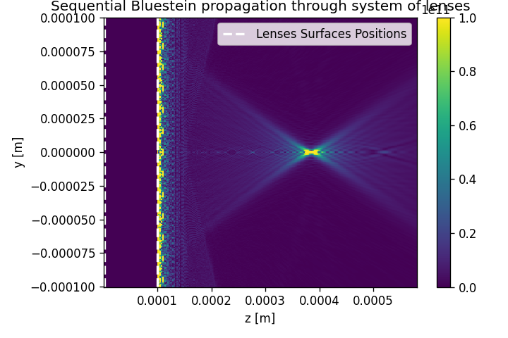
[123]:
Exy_Bluestein_all = np.hstack((np.abs(EXYZ1.screen[:,int(y_pixel/2), :])/np.max(np.abs(EXYZ1.screen[:,int(y_pixel/2), :])),\
                               np.abs(EXYZ2.screen[:,int(y_pixel/2), :])/np.max(np.abs(EXYZ2.screen[:,int(y_pixel/2), :]))))
print(Exy_Bluestein_all.shape)

zall = np.hstack((Eyz1.z, Eyz2.z+np.max(Eyz1.z) ))
yall = Eyz1.y

print(yall.shape, zall.shape)

fig = plt.figure(figsize=(7,4))
plt.pcolormesh(zall, yall, np.log(Exy_Bluestein_all) )
plt.xlabel("z [m]")
plt.ylabel("y [m]")
plt.tight_layout()

plt.vlines([zmin1+wavelength, zmin2+np.max(Eyz1.z)], -aperture_width/2, aperture_width/2, colors='white', linestyles='dashed', lw=2, \
           label="Lenses Surfaces Positions")
#plt.annotate("Fresnel distance", (limitx-limitx*0.1,-0.002), rotation="vertical", color="Red")

plt.title("Sequential ASM+Bluestein propagation through system of lenses")
plt.legend()
plt.colorbar()

plt.savefig("multilens_all_ASM-log.png", dpi=600)
(400, 400)
(400,) (400,)
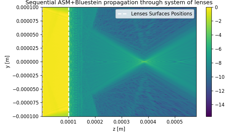
[ ]:
[124]:
##Propagate field in plane XY at z_distance using RS

z_distance = zmax1

# Creates XY screen
screen_XY = moe.field.create_screen_XY(-aperture_width/2, aperture_width/2, x_pixel,
                                       -aperture_height/2, aperture_height/2, y_pixel,
                                        z=z_distance)

# Propagate the field
E_XY = moe.propagate.RS_integral(field1, screen_XY, wavelength, simp2d=True)
Warning: Sampling field pixel is larger than wavelength/2!
[########################################] | 100% Completed | 47m 42s
[125]:
E_XY.screen[:,:,0].shape
[125]:
(400, 400)
[126]:
field2.field = E_XY.screen[:,:,0]/np.max(E_XY.screen[:,:,0])

# Modulates the field with a given aperture that can be used either as an amplitude mask or a phase mask
field2 = moe.field.modulate_field(field2, amplitude_mask = asph2_mask_inten, phase_mask=asph2_mask_phase)

# Plots the field (amplitude and phase)
moe.plotting.plot_field(field2)

plt.tight_layout()
plt.show()
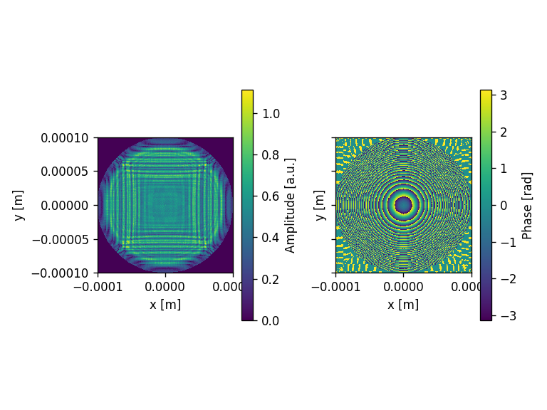
[127]:
# Propagate the field
EXYZ22 = moe.propagate.Bluestein(field2, screen2, wavelength)
Progress: [####################] 100.0%
Elapsed: 0:00:32.677759
[128]:
Eyz22 = moe.Screen(0,y2,z2)
Eyz22.screen = np.reshape(np.abs(EXYZ22.screen[:,int(y_pixel/2), :]), np.shape(Eyz2.screen[:, :, :]))

moe.plotting.plot_screen_YZ(Eyz22, which='amplitude')

limitx = moe.propagate.Fresnel_criterion(wavelength,aperture_width/2)
plt.vlines(limitx, -aperture_width/2, aperture_width/2, colors='red', linestyles='dashed', lw=2)
#plt.annotate("Fresnel distance", (limitx-limitx*0.1,-0.002), rotation="vertical", color="Red")

plt.title("|$E^2$| \n Valid for z > "+str(limitx))
plt.tight_layout()
plt.show()


Exy2 = moe.Screen(x2,y2,0)

fig = plt.figure(figsize=(5,4.5))
plt.pcolormesh(x2,y2, np.abs(EXYZ22.screen[:,:,  int(dist2/zmax2*nzs)-20]), shading='gouraud')
plt.title("Amplitude |$E$|\n  z =" +str(dist2-20*(zmax2-zmin2)/nzs))

plt.xlabel("x [m]")
plt.ylabel("y [m]")
plt.tight_layout()
plt.axis('equal')
plt.tight_layout()
plt.show()
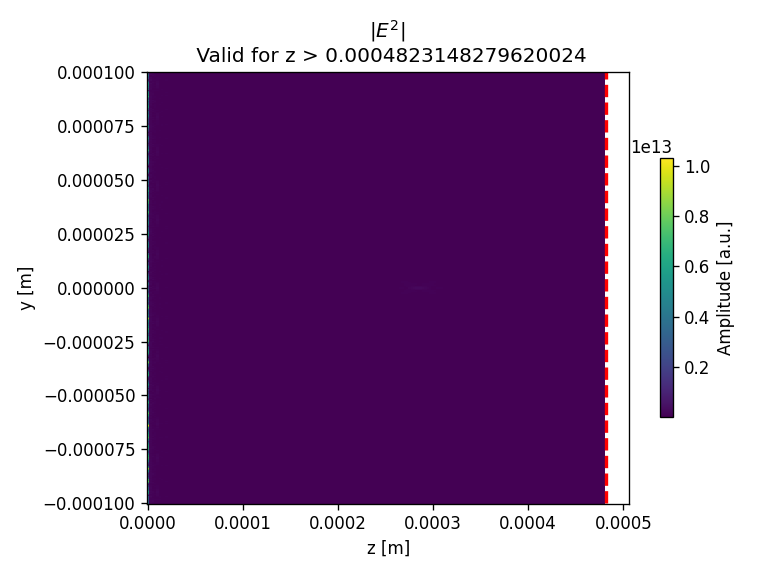
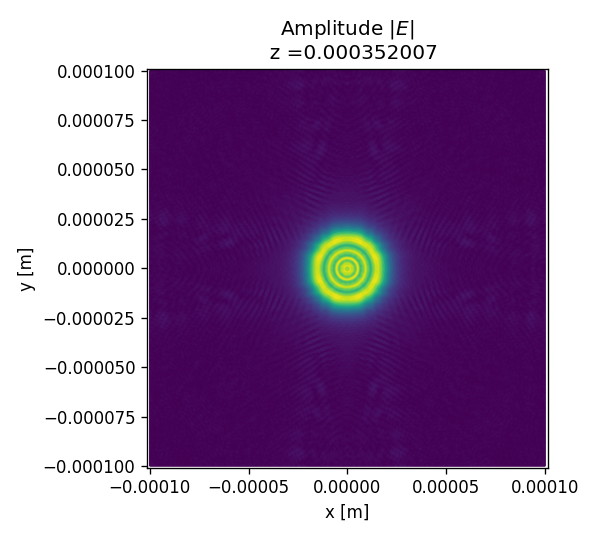
[129]:
Exy_RS_Bluestein = np.hstack((np.zeros(np.shape(np.abs(EXYZ1.screen[:,int(y_pixel/2), :]))),\
                              np.abs(EXYZ22.screen[:,int(y_pixel/2), :])))

zall = np.hstack((Eyz1.z, Eyz2.z) )
yall = Eyz1.y


fig = plt.figure(figsize=(7,4))
plt.pcolormesh(zall, yall, (Exy_RS_Bluestein), vmax=2e11)
plt.xlabel("z [m]")
plt.ylabel("y [m]")
plt.tight_layout()
plt.colorbar()

plt.vlines([zmin1+wavelength, zmin2], -aperture_width/2, aperture_width/2, colors='white', linestyles='dashed', \
           lw=2, label="Lenses Surfaces Positions")
#plt.annotate("Fresnel distance", (limitx-limitx*0.1,-0.002), rotation="vertical", color="Red")

plt.title("Sequential RS & Bluestein propagations through system of lenses")
plt.legend()

plt.savefig("multilens_RS+Bluestein.png", dpi=600)
C:\Users\jcunha377\AppData\Local\Temp\3\ipykernel_48440\4035193509.py:9: UserWarning: The input coordinates to pcolormesh are interpreted as cell centers, but are not monotonically increasing or decreasing. This may lead to incorrectly calculated cell edges, in which case, please supply explicit cell edges to pcolormesh.
  plt.pcolormesh(zall, yall, (Exy_RS_Bluestein), vmax=2e11)
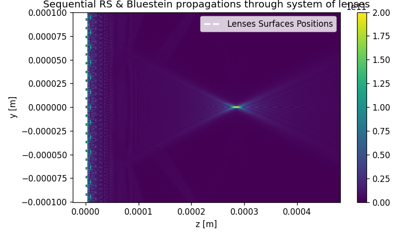
[130]:
limitx = moe.propagate.Fresnel_criterion(wavelength,aperture_width/2)
limitx
[130]:
0.0004823148279620024
[131]:
Exy_RS_Bluestein = np.hstack((np.zeros(np.shape(np.abs(EXYZ1.screen[:,int(y_pixel/2), :]))),\
                              np.abs(EXYZ22.screen[:,int(y_pixel/2), :])))

zall = np.hstack((Eyz1.z, Eyz2.z) )
yall = Eyz1.y


fig = plt.figure(figsize=(7,4))
plt.pcolormesh(zall, yall, np.log(Exy_RS_Bluestein) )
plt.xlabel("z [m]")
plt.ylabel("y [m]")
plt.tight_layout()

plt.vlines([zmin1+wavelength, zmin2], -aperture_width/2, aperture_width/2, colors='white', linestyles='dashed', \
           lw=2, label="Lenses Surfaces Positions")
#plt.annotate("Fresnel distance", (limitx-limitx*0.1,-0.002), rotation="vertical", color="Red")

plt.title("Sequential RS & Bluestein propagations through system of lenses")
plt.legend()

plt.savefig("multilens_RS+Bluestein-log.png", dpi=600)
C:\Users\jcunha377\AppData\Local\Temp\3\ipykernel_48440\1689431338.py:9: RuntimeWarning: divide by zero encountered in log
  plt.pcolormesh(zall, yall, np.log(Exy_RS_Bluestein) )
C:\Users\jcunha377\AppData\Local\Temp\3\ipykernel_48440\1689431338.py:9: UserWarning: The input coordinates to pcolormesh are interpreted as cell centers, but are not monotonically increasing or decreasing. This may lead to incorrectly calculated cell edges, in which case, please supply explicit cell edges to pcolormesh.
  plt.pcolormesh(zall, yall, np.log(Exy_RS_Bluestein) )
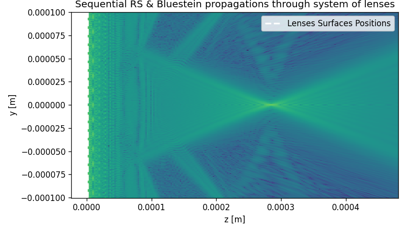
Use the ensemble class
[132]:
###Import two surfaces - doublet
import numpy as np

a1_phase = np.genfromtxt("asph1_phase.csv", delimiter=',')
a1_inten = np.genfromtxt("asph1_inten.csv", delimiter=',')

a2_phase = np.genfromtxt("asph2_phase.csv", delimiter=',')
a2_inten = np.genfromtxt("asph2_inten.csv", delimiter=',')

x_pixel, y_pixel = a1_phase.shape

print(x_pixel, y_pixel)
400 400
[133]:
#size of the rectangular mask
aperture_width  = 0.2e-3 #m
aperture_height = 0.2e-3

pixsize = 0.5e-6 #m

wavelength = 700e-9 #m

dist1 = 0.1e-3
dist2 = 0.4e-3

zmin1 = wavelength
zmax1 = dist1
nzs = 200

zmin2 = 0.1*wavelength
zmax2 = 1.2* dist2
nzs = 200
[134]:
radius = aperture_width/2


asph1_mask_phase = moe.generate.create_empty_aperture(-aperture_width/2, aperture_width/2, x_pixel, -aperture_height/2, aperture_height/2, y_pixel)
asph1_mask_phase.aperture = a1_phase

asph1_mask_inten = moe.generate.create_empty_aperture_from_aperture(asph1_mask_phase)
asph1_mask_inten.aperture = a1_inten

asph2_mask_phase = moe.generate.create_empty_aperture(-aperture_width/2, aperture_width/2, x_pixel, -aperture_height/2, aperture_height/2, y_pixel)
asph2_mask_phase.aperture = a2_phase

asph2_mask_inten = moe.generate.create_empty_aperture_from_aperture(asph2_mask_phase)
asph2_mask_inten.aperture = a2_inten

aperture = moe.generate.create_empty_aperture_from_aperture(asph2_mask_phase)
mask = moe.generate.circular_aperture(aperture, radius=radius)

aperture_array_phase = [asph1_mask_phase, asph2_mask_phase]
aperture_array_amp = [mask,]*len(aperture_array_phase)

############################
## Define the screens
x1 = asph1_mask_phase.x
y1 = asph1_mask_phase.y
z1 = np.linspace(zmin1, zmax1, nzs)

screen1 = moe.field.Screen(x1,y1,z1)

x2 = asph2_mask_phase.x
y2 = asph2_mask_phase.y
z2 = np.linspace(zmin2, zmax2, nzs)

screen2 = moe.field.Screen(x2,y2,z2)


screen_array = [screen1, screen2]

##################################
#Wavelengths
wavelength_array = [wavelength]

###############################
#input field

field_input = moe.field.create_empty_field_from_aperture(aperture)
field_input = moe.field.generate_uniform_field(field_input, E0=1)
input_light_field = field_input


##create ensemble
ensemble = moe.ensemble.Ensemble(aperture_array_amp, aperture_array_phase, screen_array,  wavelength_array, input_light_field)
[135]:
prop_methods = ["bluestein", "bluestein"]
EXY_array2 = [moe.propagate.propagate_through_ensemble(ensemble, wavelength, propagation_methods_array=prop_methods) for wavelength in wavelength_array]
Surface #1
Progress: [####################] 100.0%
Elapsed: 0:00:35.099627
Surface #2
Progress: [####################] 100.0%
Elapsed: 0:00:33.027002

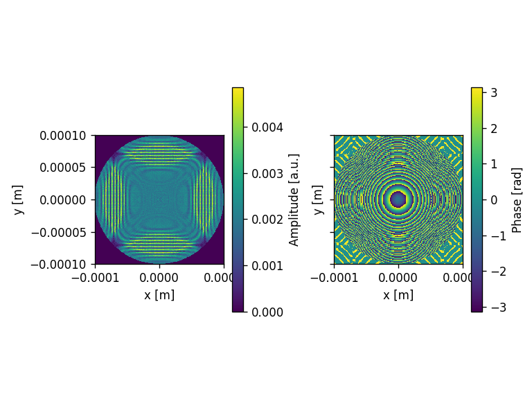
[136]:
for EXY in EXY_array2:
Exy_Bluestein_all = np.log(np.abs(EXY[:,int(y_pixel/2), :]))
zall = np.hstack((z1, z2+np.max(z1)) )
yall = y1
fig = plt.figure(figsize=(6,4))
plt.pcolormesh(zall, yall, Exy_Bluestein_all )
plt.xlabel("z [m]")
plt.ylabel("y [m]")
plt.tight_layout()
plt.vlines([zmin1+wavelength, zmin2+np.max(z1)], -aperture_width/2, aperture_width/2, colors='white', linestyles='dashed', \
lw=2, label="Lenses Surfaces Positions")
#plt.annotate("Fresnel distance", (limitx-limitx*0.1,-0.002), rotation="vertical", color="Red")
plt.title("Sequential Bluestein propagation through ensemble")
plt.legend()
#plt.savefig("multilens_all_bluestein.png", dpi=600)
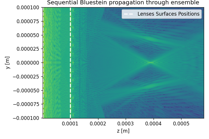
[137]:
prop_methods = ["ASM", "bluestein"]
EXY_array2 = [moe.propagate.propagate_through_ensemble(ensemble, wavelength, propagation_methods_array=prop_methods) for wavelength in wavelength_array]
Surface #1
Conventional ASM, without band limit.
Progress: [####################] 100.0%
Elapsed: 0:01:34.805522
Surface #2
Progress: [####################] 100.0%
Elapsed: 0:00:32.134204
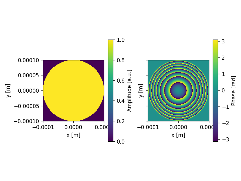

[138]:
for EXY in EXY_array2:
Exy_Bluestein_all = np.log(np.abs(EXY[:,int(y_pixel/2), :]))
zall = np.hstack((z1, z2+np.max(z1)) )
yall = y1
fig = plt.figure(figsize=(6,4))
plt.pcolormesh(zall, yall, Exy_Bluestein_all )
plt.xlabel("z [m]")
plt.ylabel("y [m]")
plt.tight_layout()
plt.vlines([zmin1+wavelength, zmin2+np.max(z1)], -aperture_width/2, aperture_width/2, colors='white', linestyles='dashed', \
lw=2, label="Lenses Surfaces Positions")
#plt.annotate("Fresnel distance", (limitx-limitx*0.1,-0.002), rotation="vertical", color="Red")
plt.title("Sequential ASM+Bluestein propagation through ensemble")
plt.legend()
#plt.savefig("multilens_all_bluestein.png", dpi=600)
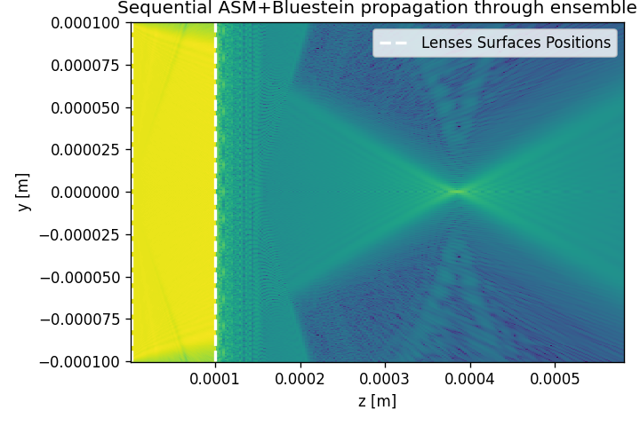
[139]:
prop_methods = ["ASM", "ASM"]
EXY_array2 = [moe.propagate.propagate_through_ensemble(ensemble, wavelength, propagation_methods_array=prop_methods) for wavelength in wavelength_array]
Surface #1
Conventional ASM, without band limit.
Progress: [####################] 100.0%
Elapsed: 0:01:30.430323
Surface #2
Conventional ASM, without band limit.
Progress: [####################] 100.0%
Elapsed: 0:01:30.239433

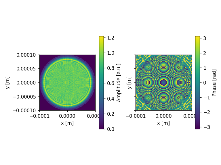
[140]:
for EXY in EXY_array2:
Exy_Bluestein_all = np.log(np.abs(EXY[:,int(y_pixel/2), :]))
zall = np.hstack((z1, z2+np.max(z1)) )
yall = y1
fig = plt.figure(figsize=(6,4))
plt.pcolormesh(zall, yall, Exy_Bluestein_all )
plt.xlabel("z [m]")
plt.ylabel("y [m]")
plt.tight_layout()
plt.vlines([zmin1+wavelength, zmin2+np.max(z1)], -aperture_width/2, aperture_width/2, colors='white', linestyles='dashed', \
lw=2, label="Lenses Surfaces Positions")
#plt.annotate("Fresnel distance", (limitx-limitx*0.1,-0.002), rotation="vertical", color="Red")
plt.title("Sequential ASM+ASM propagation through ensemble")
plt.legend()
#plt.savefig("multilens_all_bluestein.png", dpi=600)
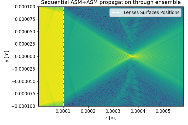
[ ]:
[ ]:
[ ]: