Example notebook for optimizer module
In the following we exemplify how to utilize the optimizer module of pyMOE which uses gradient descent methods for inverse design of masks.
The underlying idea is that the mask pixels can be iteratively refined to minimize of a loss function which evaluates the simulated propagated field from the mask against a target response. A gradient descent method changes the mask pixels iteratively in the direction of the steepest gradient until a certain tolerance is met. Some metrics can be used for loss function constructions. Examples of simple loss functions are the mean square error (MSE) or the maximum likelihood estimator. pyMOE’s
optimizer module calculates the gradient through JAX package, and employs scipy or optax (JAX) optimization frameworks, being extremelly versatile, allowing the user to pick different propagation methods (e.g. Bluestein, Scalable ASM, see propagate module example notebook) for the task.
[1]:
# Notebook display options, change as your preference/system
%matplotlib inline
%config InlineBackend.print_figure_kwargs={'facecolor' : "w",'bbox_inches':None}

import matplotlib as mpl
mpl.rcParams['figure.dpi'] = 120
[2]:
import sys
sys.path.insert(0,'..')
sys.path.insert(0,'../..')

from matplotlib import pyplot as plt
import numpy as np

from scipy.constants import micro, nano, milli

import pyMOE as moe
[3]:
# auto reload
%load_ext autoreload
%autoreload 2
[4]:
#number of pixels
x_pixel = 100
y_pixel = 100

#size of the mask
aperture_width  = 50e-6 #m
aperture_height = 50e-6

pixsize = 1e-6 #m

wavelength = 500e-9 #m
Initializations
[5]:
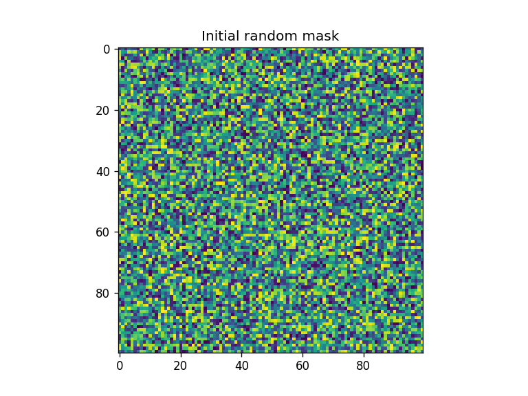
#Create initial random pixel distribution
x0 = np.random.rand(x_pixel, y_pixel)
x0_flatten = x0.flatten()

fig = plt.figure()
plt.imshow(x0)
[5]:
<matplotlib.image.AxesImage at 0x16d93442710>

[6]:
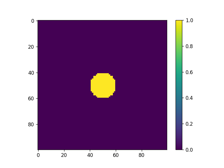
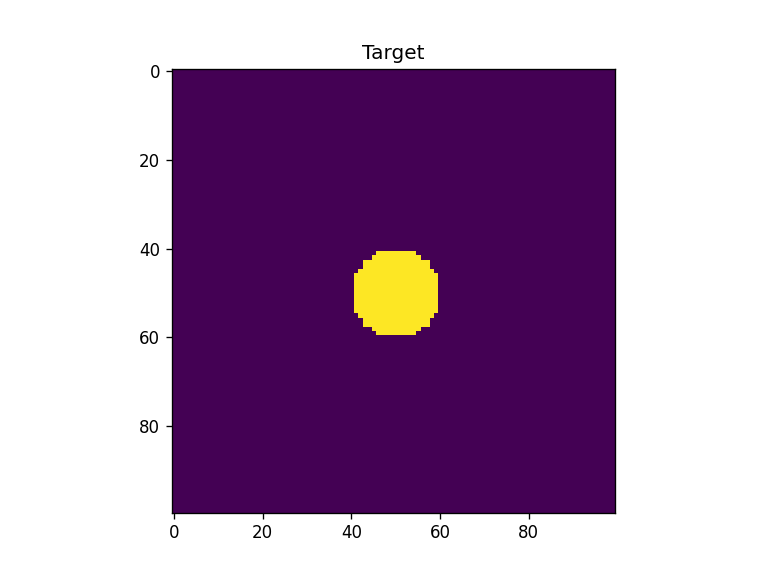
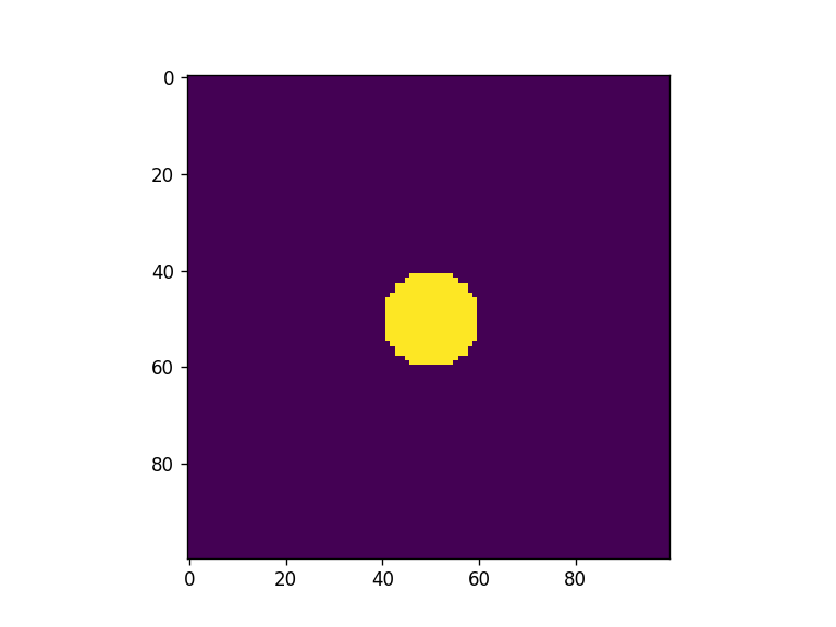
#create target matrix (central cricular pattern)
xi = np.arange(x_pixel)
yi = np.arange(y_pixel)
XX, YY = np.meshgrid(xi,yi)

target = np.zeros((x_pixel, y_pixel))
target[np.where(((XX-x_pixel/2)**2 + (YY-y_pixel/2)**2) < 10**2)] = 1

target_flat = target.flatten()

fig = plt.figure()
plt.imshow(target)
plt.colorbar()
[6]:
<matplotlib.colorbar.Colorbar at 0x16d94cfd550>
Optimization framework
The optimization framework passes through the definition of loss functions. Here simply they compare the propagation against a defined target. The loss function takes the propagation method as parameter, so that different propagators can be tested.
[7]:
#Define loss functions
def mseloss(x, mask, screen, wavelength, target, propag="bluestein"):
    import jax.numpy as jnp

    prop_x =  jnp.abs(moe.optimizer.propagate(jnp.reshape(x, (len(screen.x), len(screen.y))), mask, screen, wavelength, propagation_method=propag))

    diff = jnp.abs(prop_x/jnp.sum(prop_x) - target/jnp.max(target))**2

    res = jnp.mean(diff)

    return res


def logloss(x, mask, screen, wavelength, target=target_flat, propag="bluestein", use_timer=True):
    import jax.numpy as jnp

    prop_x = jnp.abs(moe.optimizer.propagate(jnp.reshape(x, (x_pixel, y_pixel)), mask, screen, wavelength, propagation_method=propag, use_timer=use_timer).flatten())
    prop_x = jnp.reshape(prop_x, (x_pixel, y_pixel))
    midx, midy = int(x_pixel/2), int(y_pixel/2)
    target = jnp.reshape(target, (x_pixel, y_pixel))

    res = jnp.log(np.sum(((prop_x/jnp.max(prop_x)/(prop_x[(midx,midy)]/jnp.max(prop_x)) - target/jnp.max(target))**2)))

    return res
[8]:
# Create Aperture
aperture = moe.generate.create_empty_aperture(-aperture_width/2, aperture_width/2, x_pixel, -aperture_height/2, aperture_height/2, y_pixel)
[9]:
# Creates a screen in YZ plane with [-aperture_height/2, aperture_height/2] at zdist
ymin, ymax = -aperture_height/2, aperture_height/2
xmin, xmax = -aperture_width/2, aperture_width/2

zdist = 0.00015

x = np.linspace(xmin, xmax, x_pixel)
y = np.linspace(ymin, ymax, y_pixel)
z = np.array([zdist])

screen = moe.Screen(x,y,z)
[10]:
#optimize using the optimizer module  and Bluestein propagation (default)
# the initial guess is the randomly initialized x0
solution = moe.optimizer.optimize(mseloss, x0_flatten, args1=[aperture, screen, wavelength, target], verbose = 1, ftol=1e-4, )
Elapsed: 0:00:00.993681
Elapsed: 0:00:00.018917
Elapsed: 0:00:00.275790
Elapsed: 0:00:00.015929
Elapsed: 0:00:00.013938
Elapsed: 0:00:00.039850
Elapsed: 0:00:00.013939
Elapsed: 0:00:00.013939
Elapsed: 0:00:00.037834
Elapsed: 0:00:00.014935
Elapsed: 0:00:00.013941
Elapsed: 0:00:00.037834
Elapsed: 0:00:00.013937
Elapsed: 0:00:00.013937
Elapsed: 0:00:00.037834
Elapsed: 0:00:00.014935
Elapsed: 0:00:00.013465
Elapsed: 0:00:00.047789
Elapsed: 0:00:00.014935
Elapsed: 0:00:00.012943
Elapsed: 0:00:00.042812
Elapsed: 0:00:00.014935
Elapsed: 0:00:00.013939
Elapsed: 0:00:00.039825
Elapsed: 0:00:00.013939
Elapsed: 0:00:00.013939
Elapsed: 0:00:00.051773
Elapsed: 0:00:00.013939
Elapsed: 0:00:00.013939
Elapsed: 0:00:00.037834
Elapsed: 0:00:00.016926
Elapsed: 0:00:00.016926
Elapsed: 0:00:00.037834
Elapsed: 0:00:00.013938
Elapsed: 0:00:00.013938
Elapsed: 0:00:00.037833
Elapsed: 0:00:00.013938
Elapsed: 0:00:00.013939
Elapsed: 0:00:00.040821
Elapsed: 0:00:00.014935
Elapsed: 0:00:00.014934
Elapsed: 0:00:00.040823
Elapsed: 0:00:00.013939
Elapsed: 0:00:00.013940
Elapsed: 0:00:00.055755
Elapsed: 0:00:00.013938
Elapsed: 0:00:00.012943
Elapsed: 0:00:00.037835
Elapsed: 0:00:00.013939
Elapsed: 0:00:00.013939
Elapsed: 0:00:00.039825
Elapsed: 0:00:00.013939
Elapsed: 0:00:00.013933
Elapsed: 0:00:00.040820
`ftol` termination condition is satisfied.
Function evaluations 18, initial cost 4.6493e-04, final cost 4.6108e-04, first-order optimality 4.44e-09.
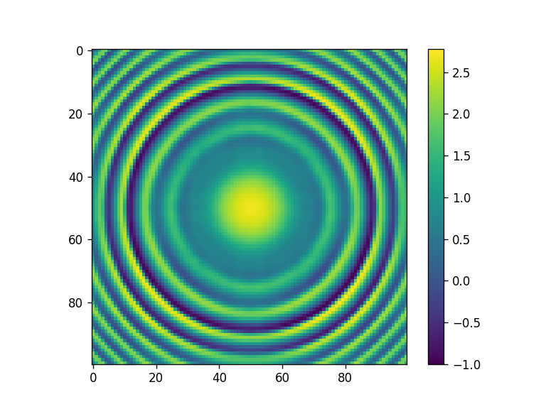
[11]:
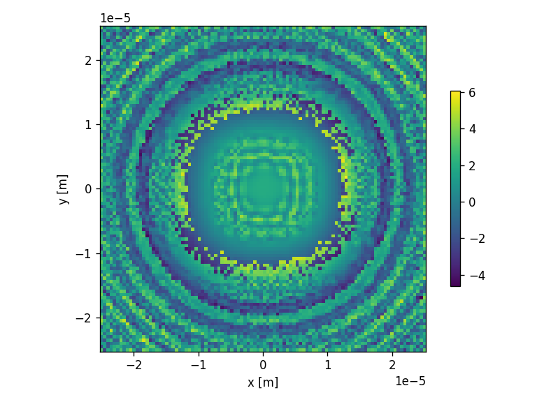
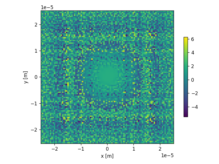
x = solution.x
xar = np.reshape(x, (x_pixel, y_pixel))

#just for plotting the phase with dimensions
aperture.aperture = xar
moe.plotting.plot_aperture(aperture)
[12]:
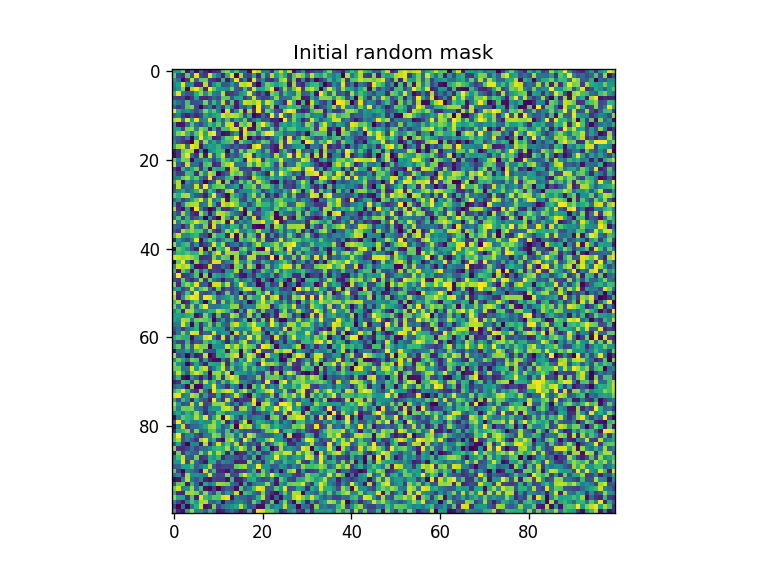
fig = plt.figure()
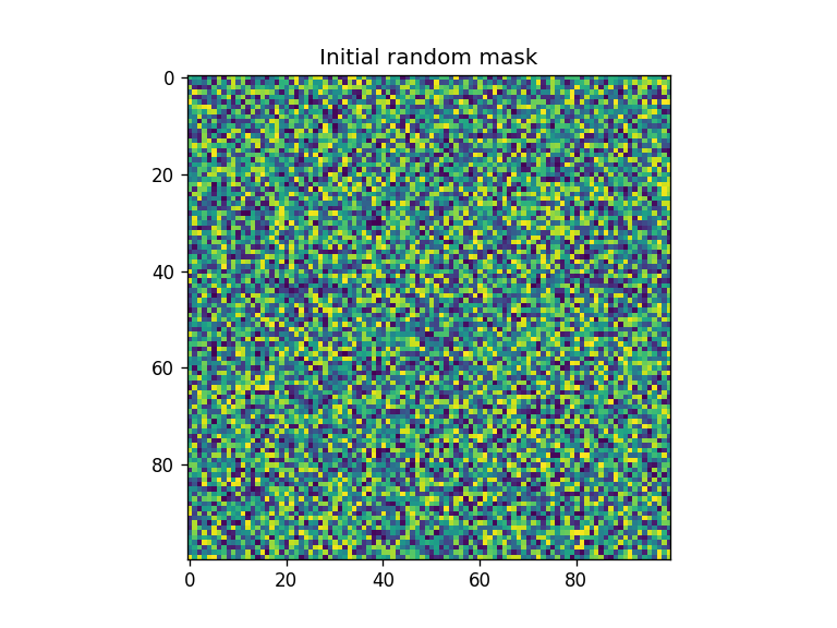
xar2 = np.reshape(x0_flatten, (x_pixel, y_pixel))
plt.imshow(xar2)
plt.title("Initial random mask")
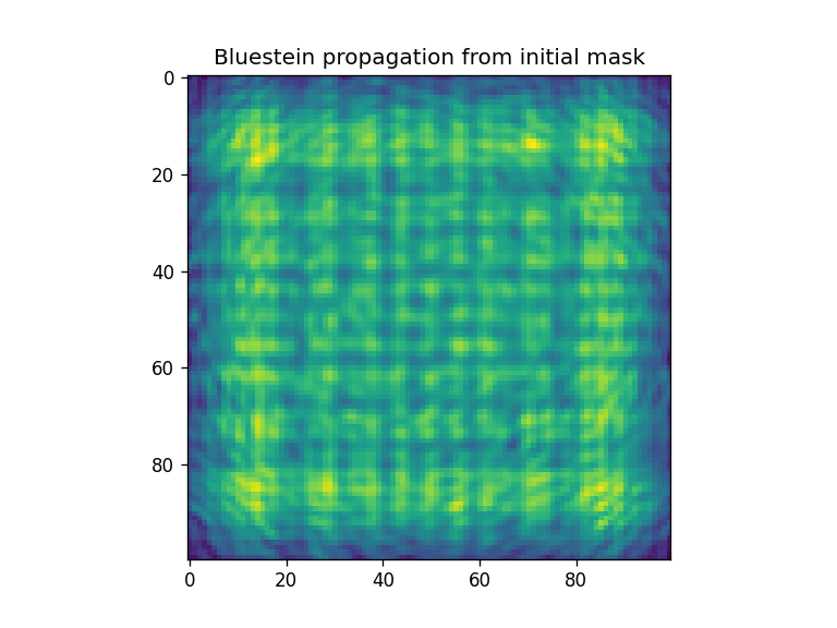
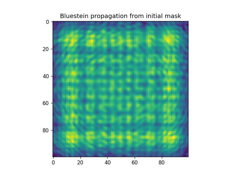
fig = plt.figure()
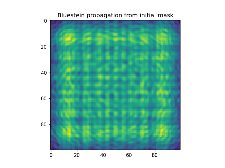
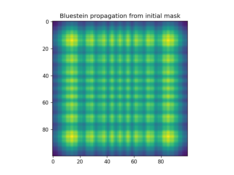
plt.imshow(np.abs(moe.optimizer.propagate(xar2, aperture, screen, wavelength) ) )
plt.title("Bluestein propagation from initial mask")
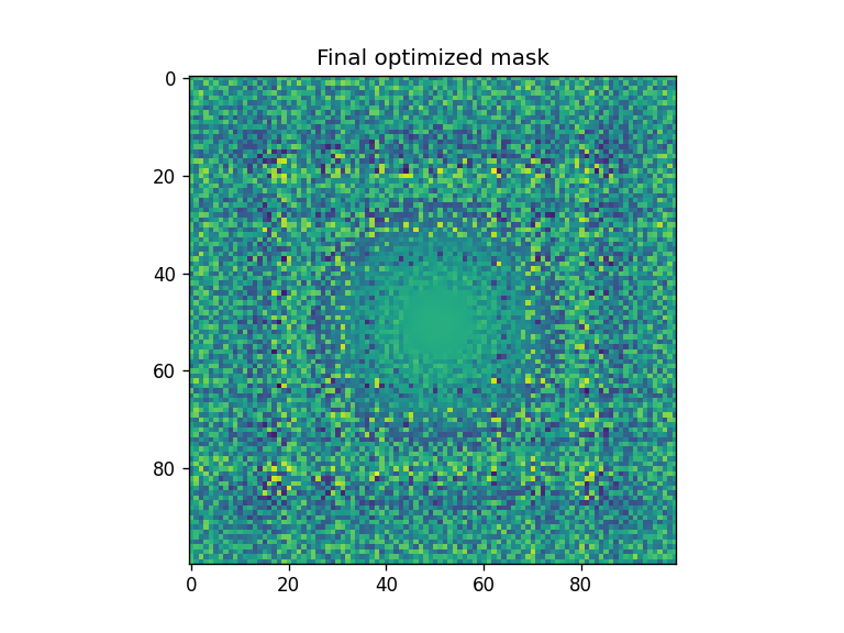
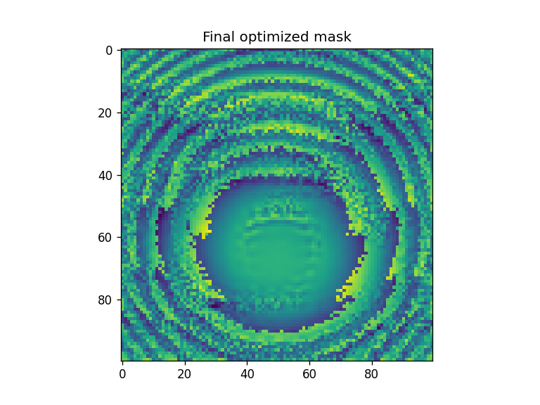
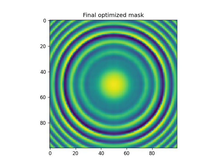
fig = plt.figure()
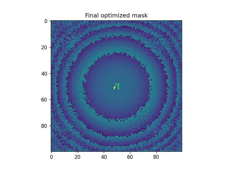
xar3 = np.reshape(x, (x_pixel, y_pixel))
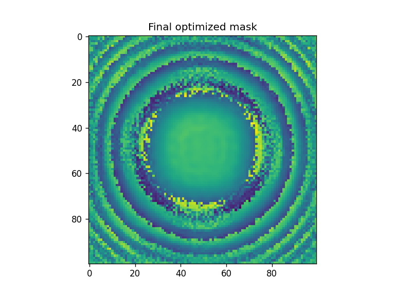
plt.imshow(xar3)
plt.title("Final optimized mask")
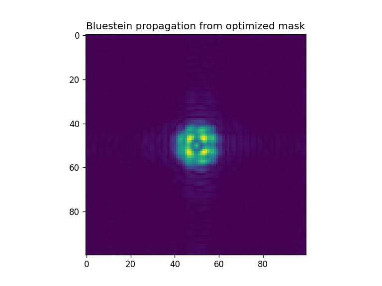
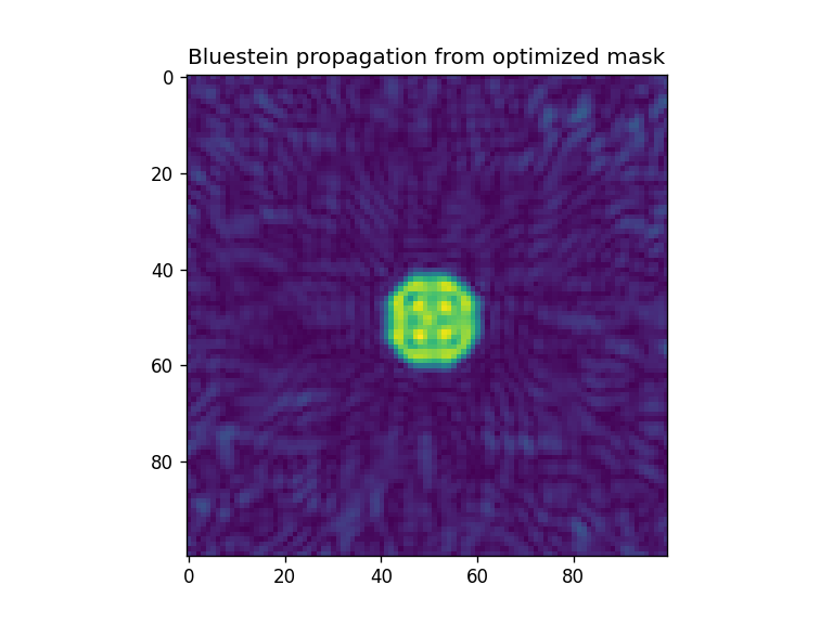
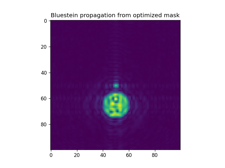
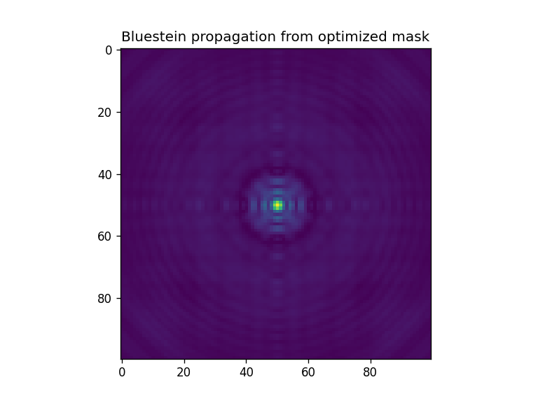
fig = plt.figure()
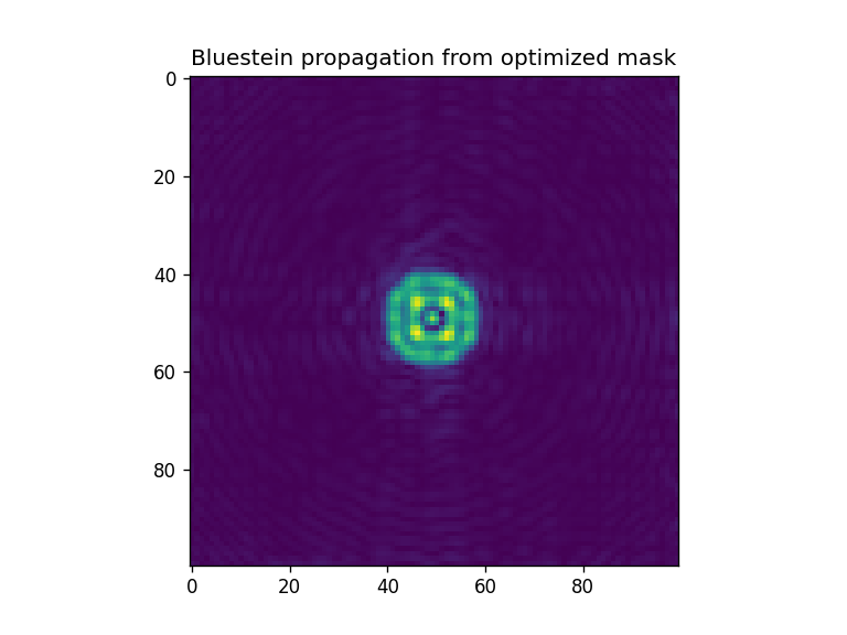
plt.imshow(np.abs(moe.optimizer.propagate(xar3, aperture, screen, wavelength) ) )
plt.title("Bluestein propagation from optimized mask")
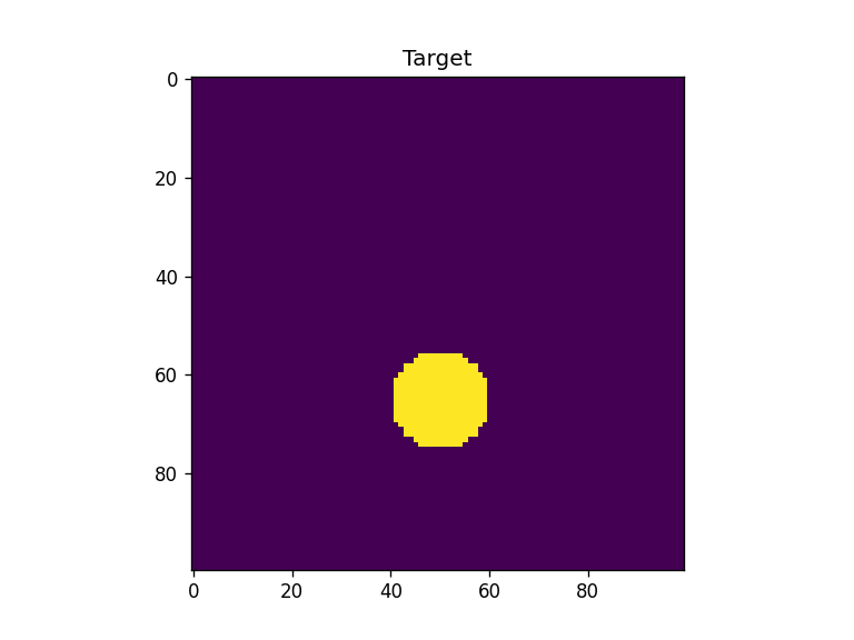
fig = plt.figure()
plt.imshow(np.reshape(target, (x_pixel, y_pixel)) )
plt.title("Target")
Elapsed: 0:00:00.014935
Elapsed: 0:00:00.024890
[12]:
Text(0.5, 1.0, 'Target')


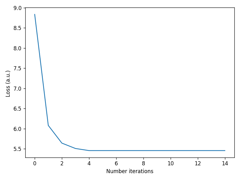
[13]:
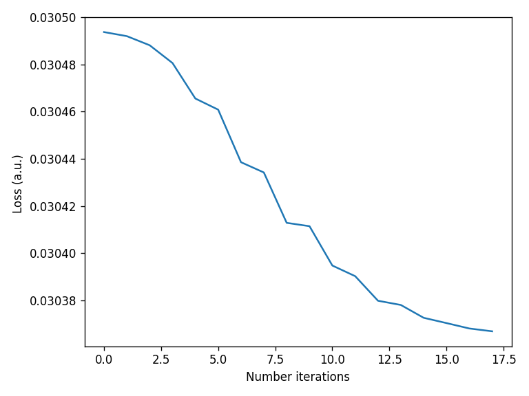
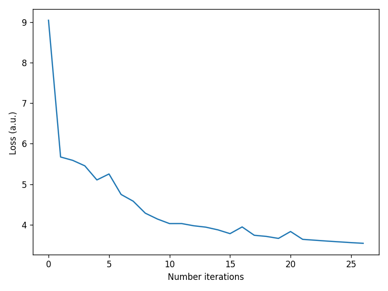
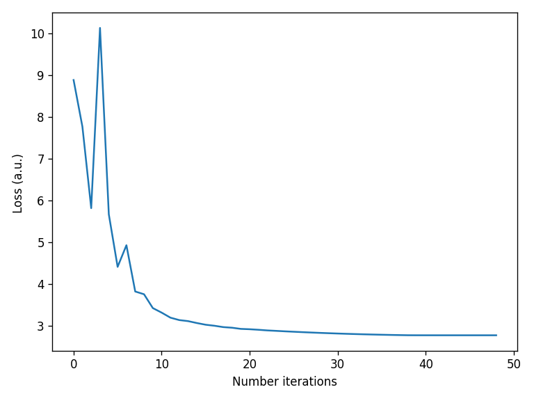
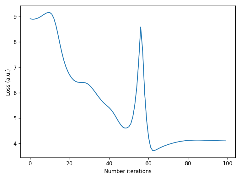
loss_vector = solution.loss_history

plt.figure()
plt.plot(loss_vector)
plt.xlabel("Number iterations")
plt.ylabel("Loss (a.u.) ")
plt.tight_layout()

Optimization with logging
The optimizermodule provides an embedded logger to allow to track the optimization loss and store the parameters at each iteration step.
[14]:
# x0_flatten is your initial guess vector
logger, logfile_txt, logfile_bin, batch_list, iter_counter, batch_size, fh = moe.optimizer.setup_optimizer_logger_batch( x_size=len(x0_flatten), \
                                                                                                       batch_size=1, log_dir="logs", name="test")
[15]:
#optimize using the optimizer module  and Bluestein propagation (default)
# the initial guess is the randomly initialized x0
solution = moe.optimizer.optimize(mseloss, x0_flatten, args1=[aperture, screen, wavelength, target], verbose = 1, ftol=1e-4, logger=logger, \
                                  logfile_bin=logfile_bin, batch_list=batch_list, batch_size=batch_size, iter_counter=iter_counter, fh=fh)
Elapsed: 0:00:00.016926
Elapsed: 0:00:00.013938
Elapsed: 0:00:00.041817
Elapsed: 0:00:00.018917
Elapsed: 0:00:00.017921
Elapsed: 0:00:00.051773
Elapsed: 0:00:00.017922
Elapsed: 0:00:00.017922
Elapsed: 0:00:00.043828
Elapsed: 0:00:00.013937
Elapsed: 0:00:00.018916
Elapsed: 0:00:00.037834
Elapsed: 0:00:00.013933
Elapsed: 0:00:00.025886
Elapsed: 0:00:00.060733
Elapsed: 0:00:00.013938
Elapsed: 0:00:00.016925
Elapsed: 0:00:00.038829
Elapsed: 0:00:00.019912
Elapsed: 0:00:00.016925
Elapsed: 0:00:00.038830
Elapsed: 0:00:00.013938
Elapsed: 0:00:00.013938
Elapsed: 0:00:00.037834
Elapsed: 0:00:00.016927
Elapsed: 0:00:00.013939
Elapsed: 0:00:00.038830
Elapsed: 0:00:00.012944
Elapsed: 0:00:00.015930
Elapsed: 0:00:00.037855
Elapsed: 0:00:00.013939
Elapsed: 0:00:00.013939
Elapsed: 0:00:00.038831
Elapsed: 0:00:00.013939
Elapsed: 0:00:00.014972
Elapsed: 0:00:00.037835
Elapsed: 0:00:00.014935
Elapsed: 0:00:00.014934
Elapsed: 0:00:00.039825
Elapsed: 0:00:00.013938
Elapsed: 0:00:00.014934
Elapsed: 0:00:00.037834
Elapsed: 0:00:00.017920
Elapsed: 0:00:00.024891
Elapsed: 0:00:00.037857
Elapsed: 0:00:00.014934
Elapsed: 0:00:00.018917
Elapsed: 0:00:00.037828
Elapsed: 0:00:00.013938
Elapsed: 0:00:00.015931
Elapsed: 0:00:00.040820
Elapsed: 0:00:00.013939
Elapsed: 0:00:00.025887
Elapsed: 0:00:00.054759
`ftol` termination condition is satisfied.
Function evaluations 18, initial cost 4.6493e-04, final cost 4.6108e-04, first-order optimality 4.44e-09.
[16]:
x = solution.x
xar = np.reshape(x, (x_pixel, y_pixel))

fig = plt.figure()
xar2 = np.reshape(x0_flatten, (x_pixel, y_pixel))
plt.imshow(xar2)
plt.title("Initial random mask")

fig = plt.figure()
plt.imshow(np.abs(moe.optimizer.propagate(xar2, aperture, screen, wavelength) ) )
plt.title("Bluestein propagation from initial mask")


fig = plt.figure()
xar3 = np.reshape(x, (x_pixel, y_pixel))
plt.imshow(xar3)
plt.title("Final optimized mask")

fig = plt.figure()
plt.imshow(np.abs(moe.optimizer.propagate(xar3, aperture, screen, wavelength) ) )
plt.title("Bluestein propagation from optimized mask")

fig = plt.figure()
plt.imshow(np.reshape(target, (x_pixel, y_pixel)) )
plt.title("Target")
Elapsed: 0:00:00.014935
Elapsed: 0:00:00.014934
[16]:
Text(0.5, 1.0, 'Target')


[17]:
loss_vector = solution.loss_history

plt.figure()
plt.plot(loss_vector)
plt.xlabel("Number iterations")
plt.ylabel("Loss (a.u.) ")
plt.tight_layout()
Optimization with different forward propagators
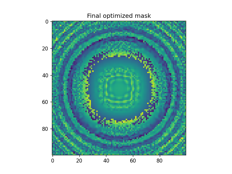
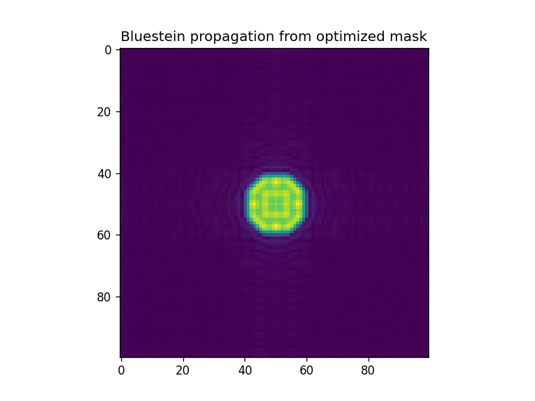
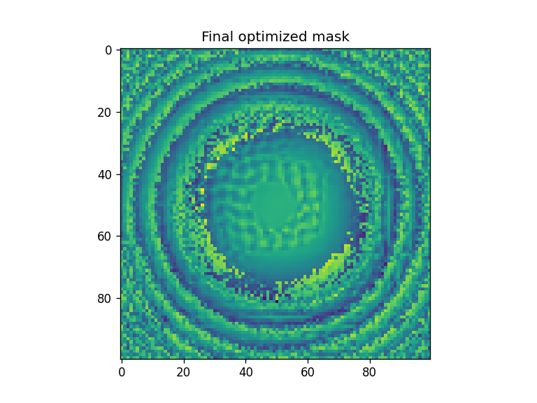
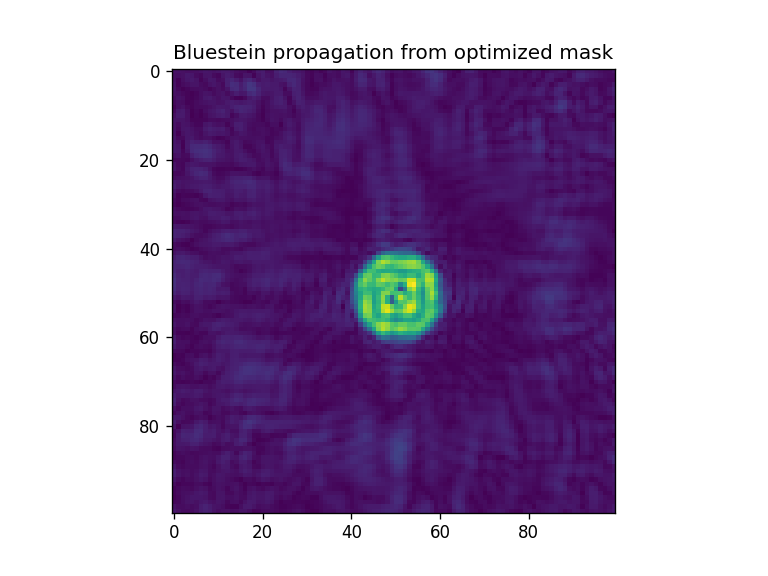
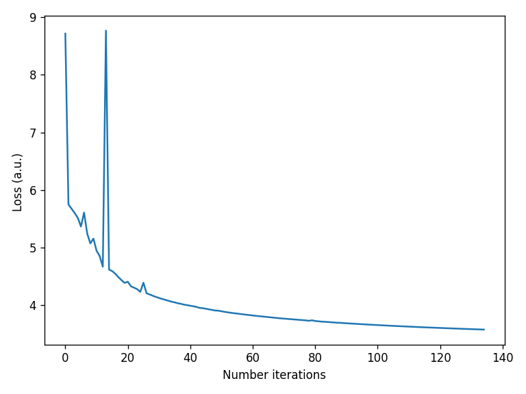
Below we demonstrate several optimizations using Bluestein, ASM and SASM propagators in the forward step. All of them yield acceptable inverse designed masks.
Bluestein (default)
[18]:
#optimize using the optimizer module  and Bluestein propagation (default)
# the initial guess is the randomly initialized x0
solution = moe.optimizer.optimize(logloss, x0_flatten, args1=[aperture, screen, wavelength, target, "bluestein", False], verbose = 1, ftol=1e-4)
`ftol` termination condition is satisfied.
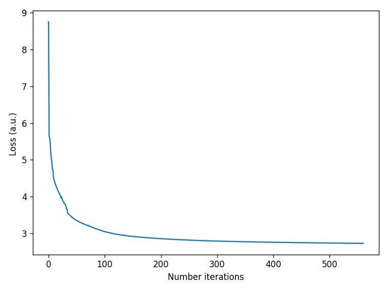
Function evaluations 561, initial cost 3.8314e+01, final cost 3.7114e+00, first-order optimality 9.27e-04.
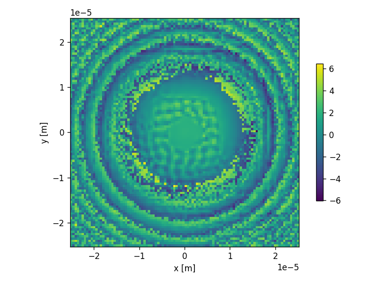
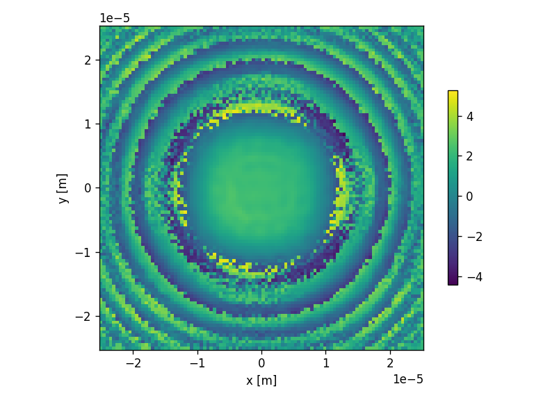
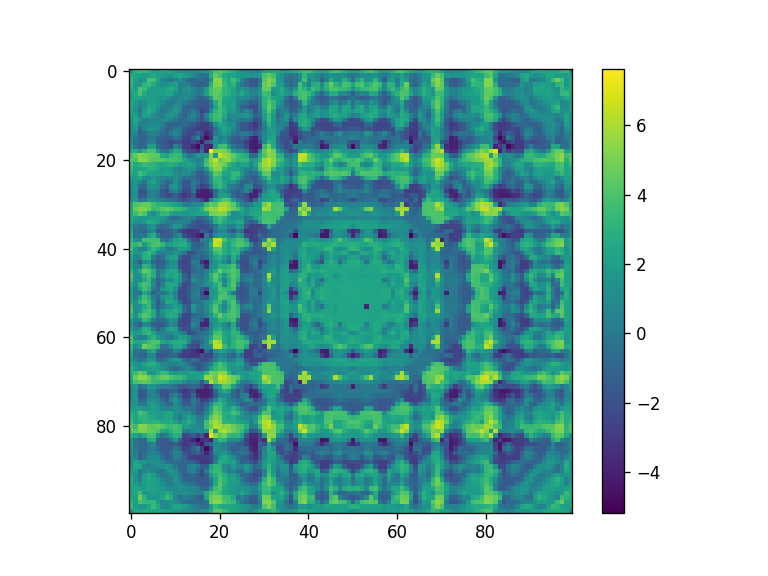
[19]:
x = solution.x
xar = np.reshape(x, (x_pixel, y_pixel))

#just for plotting the phase with dimensions
aperture.aperture = xar
moe.plotting.plot_aperture(aperture)
[20]:
fig = plt.figure()
xar2 = np.reshape(x0_flatten, (x_pixel, y_pixel))
plt.imshow(xar2)
plt.title("Initial random mask")

fig = plt.figure()
plt.imshow(np.abs(moe.optimizer.propagate(xar2, aperture, screen, wavelength) ) )
plt.title("Bluestein propagation from initial mask")


fig = plt.figure()
xar3 = np.reshape(x, (x_pixel, y_pixel))
plt.imshow(xar3)
plt.title("Final optimized mask")

fig = plt.figure()
plt.imshow(np.abs(moe.optimizer.propagate(xar3, aperture, screen, wavelength) ) )
plt.title("Bluestein propagation from optimized mask")

fig = plt.figure()
plt.imshow(np.reshape(target, (x_pixel, y_pixel)) )
plt.title("Target")
Elapsed: 0:00:00.015929
Elapsed: 0:00:00.013938
[20]:
Text(0.5, 1.0, 'Target')


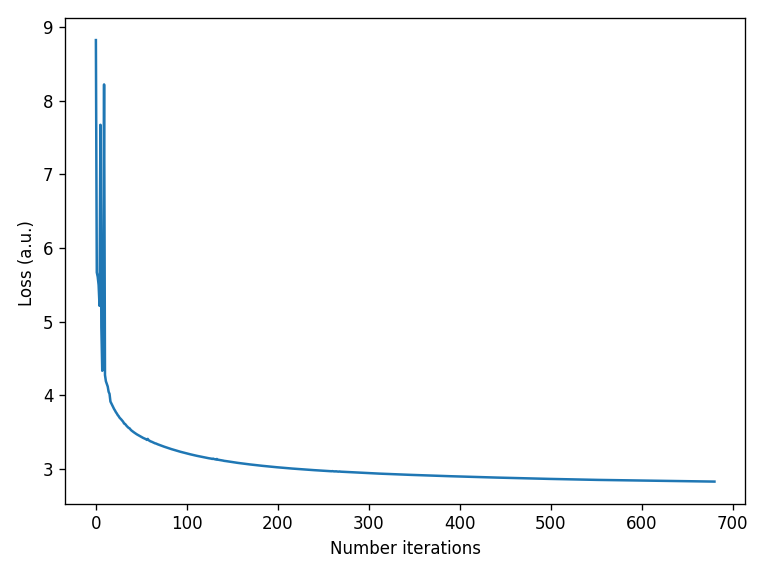
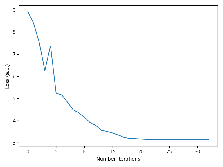
[21]:
loss_vector = solution.loss_history

plt.figure()
plt.plot(loss_vector)
plt.xlabel("Number iterations")
plt.ylabel("Loss (a.u.) ")
plt.tight_layout()
ASM
[22]:
#optimize using the optimizer module  and Bluestein propagation (default)
# the initial guess is the randomly initialized x0
solution = moe.optimizer.optimize(logloss, x0_flatten, args1=[aperture, screen, wavelength, target, "ASM", False], verbose = 1, ftol=1e-4,)
C:\Users\jcunha377\AppData\Roaming\Python\Python311\site-packages\jax\_src\numpy\lax_numpy.py:148: UserWarning: Explicitly requested dtype complex128 requested in asarray is not available, and will be truncated to dtype complex64. To enable more dtypes, set the jax_enable_x64 configuration option or the JAX_ENABLE_X64 shell environment variable. See https://github.com/google/jax#current-gotchas for more.
  return asarray(x, dtype=self.dtype)
`ftol` termination condition is satisfied.
Function evaluations 681, initial cost 3.8899e+01, final cost 3.9955e+00, first-order optimality 8.61e-04.
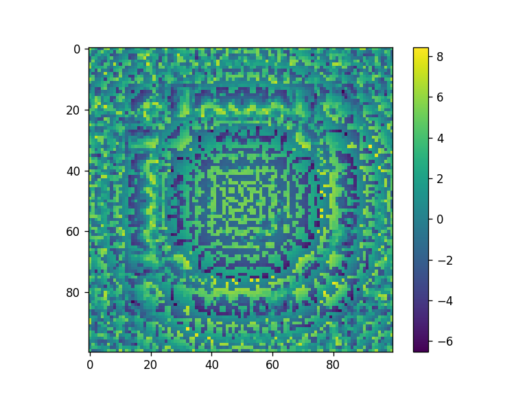
[23]:
x = solution.x
xar = np.reshape(x, (x_pixel, y_pixel))

#just for plotting the phase with dimensions
aperture.aperture = xar
moe.plotting.plot_aperture(aperture)
[24]:
fig = plt.figure()
xar2 = np.reshape(x0_flatten, (x_pixel, y_pixel))
plt.imshow(xar2)
plt.title("Initial random mask")

fig = plt.figure()
plt.imshow(np.abs(moe.optimizer.propagate(xar2, aperture, screen, wavelength) ) )
plt.title("Bluestein propagation from initial mask")


fig = plt.figure()
xar3 = np.reshape(x, (x_pixel, y_pixel))
plt.imshow(xar3)
plt.title("Final optimized mask")

fig = plt.figure()
plt.imshow(np.abs(moe.optimizer.propagate(xar3, aperture, screen, wavelength) ) )
plt.title("Bluestein propagation from optimized mask")

fig = plt.figure()
plt.imshow(np.reshape(target, (x_pixel, y_pixel)) )
plt.title("Target")
Elapsed: 0:00:00.015930
Elapsed: 0:00:00.024893
[24]:
Text(0.5, 1.0, 'Target')


[25]:
loss_vector = solution.loss_history

plt.figure()
plt.plot(loss_vector)
plt.xlabel("Number iterations")
plt.ylabel("Loss (a.u.) ")
plt.tight_layout()
SASM
[26]:
#optimize using the optimizer module  and Bluestein propagation (default)
# the initial guess is the randomly initialized x0
solution = moe.optimizer.optimize(logloss, x0_flatten, args1=[aperture, screen, wavelength, target, "SASM", False], verbose = 1, ftol=1e-2,)
`ftol` termination condition is satisfied.
Function evaluations 27, initial cost 4.0914e+01, final cost 6.2704e+00, first-order optimality 4.19e-03.
[27]:
x = solution.x
xar = np.reshape(x, (x_pixel, y_pixel))

#just for plotting the phase with dimensions
aperture.aperture = xar
moe.plotting.plot_aperture(aperture)
[28]:
fig = plt.figure()
xar2 = np.reshape(x0_flatten, (x_pixel, y_pixel))
plt.imshow(xar2)
plt.title("Initial random mask")

fig = plt.figure()
plt.imshow(np.abs(moe.optimizer.propagate(xar2, aperture, screen, wavelength) ) )
plt.title("Bluestein propagation from initial mask")


fig = plt.figure()
xar3 = np.reshape(x, (x_pixel, y_pixel))
plt.imshow(xar3)
plt.title("Final optimized mask")

fig = plt.figure()
plt.imshow(np.abs(moe.optimizer.propagate(xar3, aperture, screen, wavelength) ) )
plt.title("Bluestein propagation from optimized mask")

fig = plt.figure()
plt.imshow(np.reshape(target, (x_pixel, y_pixel)) )
plt.title("Target")
Elapsed: 0:00:00.014933
Elapsed: 0:00:00.013939
[28]:
Text(0.5, 1.0, 'Target')


[29]:
loss_vector = solution.loss_history

plt.figure()
plt.plot(loss_vector)
plt.xlabel("Number iterations")
plt.ylabel("Loss (a.u.) ")
plt.tight_layout()
Loss function engineering
We can alter the loss function for whatever suits us best
[30]:
def logloss2(x, mask, screen, wavelength, target, propag, use_timer):
    import jax.numpy as jnp

    prop_x =  jnp.abs(moe.optimizer.propagate(np.reshape(x, (len(screen.x), len(screen.y))), mask, screen, wavelength, propagation_method=propag , use_timer=use_timer))

    diff = jnp.abs(prop_x/prop_x[int(len(screen.x)/2), int(len(screen.y)/2)] - target/jnp.max(target))**2

    res = jnp.log(jnp.sum(diff))

    return res
[31]:
## Optimization with ASM
x0 = np.random.rand(x_pixel, y_pixel)
x0_flatten = x0.flatten()

x = np.linspace(xmin, xmax, x_pixel)
y = np.linspace(ymin, ymax, y_pixel)
z = np.array([zdist])

screen = moe.Screen(x,y,z)

aperture = moe.generate.create_empty_aperture(-aperture_width/2, aperture_width/2, x_pixel, -aperture_height/2, aperture_height/2, y_pixel)

solution = moe.optimizer.optimize(logloss2, x0_flatten, args1=[aperture, screen, wavelength, target, "ASM", False], verbose = 1, ftol=1e-3,)
`xtol` termination condition is satisfied.
Function evaluations 49, initial cost 3.9489e+01, final cost 3.8438e+00, first-order optimality 3.19e-03.
[32]:
x = solution.x
xar = np.reshape(x, (x_pixel, y_pixel))

#just for plotting the phase with dimensions
aperture.aperture = xar
moe.plotting.plot_aperture(aperture)
[33]:
fig = plt.figure()
xar2 = np.reshape(x0_flatten, (x_pixel, y_pixel))
plt.imshow(xar2)
plt.title("Initial random mask")

fig = plt.figure()
plt.imshow(np.abs(moe.optimizer.propagate(xar2, aperture, screen, wavelength) ) )
plt.title("Bluestein propagation from initial mask")


fig = plt.figure()
xar3 = np.reshape(x, (x_pixel, y_pixel))
plt.imshow(xar3)
plt.title("Final optimized mask")

fig = plt.figure()
plt.imshow(np.abs(moe.optimizer.propagate(xar3, aperture, screen, wavelength) ) )
plt.title("Bluestein propagation from optimized mask")

fig = plt.figure()
plt.imshow(np.reshape(target, (x_pixel, y_pixel)) )
plt.title("Target")
Elapsed: 0:00:00.023896
Elapsed: 0:00:00.013939
[33]:
Text(0.5, 1.0, 'Target')
[34]:
loss_vector = solution.loss_history

plt.figure()
plt.plot(loss_vector)
plt.xlabel("Number iterations")
plt.ylabel("Loss (a.u.) ")
plt.tight_layout()
Target re-definition
We can alter the target for what we desire. The target can be generated from analytical or theoretical models, e.g. it could be generated as Airy pattern or Gaussian-Laguerre beam profile.
[35]:
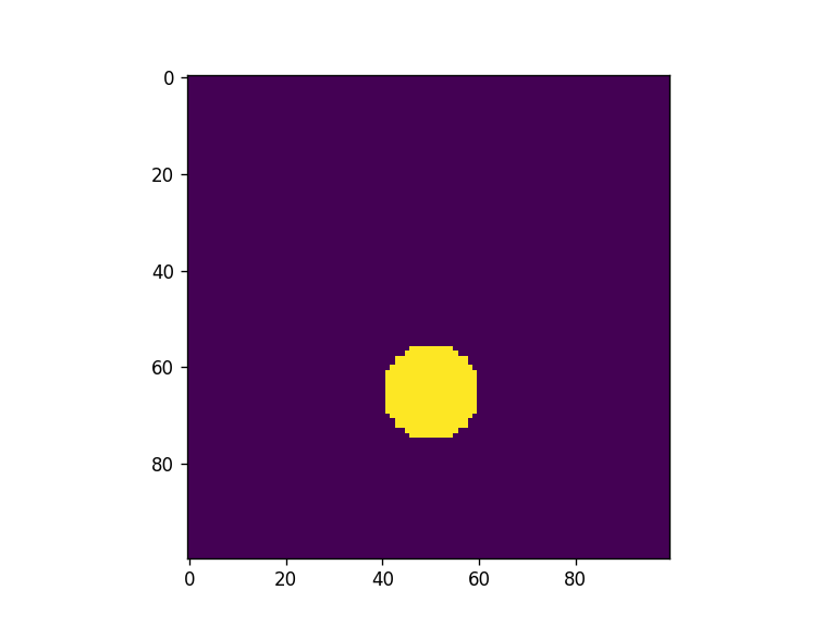
# re-define  target

#target with offset circle
xi = np.arange(x_pixel)
yi = np.arange(y_pixel*2)
XX, YY = np.meshgrid(xi,yi)

target = np.zeros((x_pixel, y_pixel))
target[np.where(((XX-x_pixel/2- 0)**2 + (YY-y_pixel/2-15)**2) < 10**2)] = 1


fig = plt.figure()
plt.imshow(target)
[35]:
<matplotlib.image.AxesImage at 0x16da5cf6110>
[36]:
## Optimization with ASM
x0 = np.random.rand(x_pixel, y_pixel)
x0_flatten = x0.flatten()

x = np.linspace(xmin, xmax, x_pixel)
y = np.linspace(ymin, ymax, y_pixel)
z = np.array([zdist])

screen = moe.Screen(x,y,z)

aperture = moe.generate.create_empty_aperture(-aperture_width/2, aperture_width/2, x_pixel, -aperture_height/2, aperture_height/2, y_pixel)
[37]:
solution = moe.optimizer.optimize(logloss2, x0_flatten, args1=[aperture, screen, wavelength, target, "bluestein", False], verbose = 1, ftol=1e-3,)

x = solution.x
`ftol` termination condition is satisfied.
Function evaluations 135, initial cost 3.7973e+01, final cost 6.3892e+00, first-order optimality 2.94e-03.
[38]:
xar = np.reshape(x, (x_pixel, y_pixel))
[39]:
fig = plt.figure()
xar2 = np.reshape(x0_flatten, (x_pixel, y_pixel))
plt.imshow(xar2)
plt.title("Initial random mask")

fig = plt.figure()
plt.imshow(np.abs(moe.optimizer.propagate(xar2, aperture, screen, wavelength) ) )
plt.title("Bluestein propagation from initial mask")


fig = plt.figure()
xar3 = np.reshape(x, (x_pixel, y_pixel))
plt.imshow(xar3)
plt.title("Final optimized mask")

fig = plt.figure()
plt.imshow(np.abs(moe.optimizer.propagate(xar3, aperture, screen, wavelength) ) )
plt.title("Bluestein propagation from optimized mask")

fig = plt.figure()
plt.imshow(np.reshape(target, (x_pixel, y_pixel)) )
plt.title("Target")
Elapsed: 0:00:00.019914
Elapsed: 0:00:00.015930
[39]:
Text(0.5, 1.0, 'Target')
[40]:
loss_vector = solution.loss_history

plt.figure()
plt.plot(loss_vector)
plt.xlabel("Number iterations")
plt.ylabel("Loss (a.u.) ")
plt.tight_layout()
Other optimizer algorithms
By default the optimize function uses the ‘trf’ scipy algorithm. Here we exemplify ‘dogbox’ method as well. Other optimization algortihms can be used as well, namely all methods in scipy minimize, and ‘adam’ and ‘rmsprop’ from JAX’ optax package.
[41]:
### Testing constant value initial guess

#Initial guess
x0 = np.ones((x_pixel,y_pixel))
x0_flatten = x0.flatten()


#create target matrix (central cricular pattern)
xi = np.arange(x_pixel)
yi = np.arange(y_pixel)
XX, YY = np.meshgrid(xi,yi)

target = np.zeros((x_pixel, y_pixel))
target[np.where(((XX-x_pixel/2)**2 + (YY-y_pixel/2)**2) < 10**2)] = 1

target_flat = target.flatten()

fig = plt.figure()
plt.imshow(target)
[41]:
<matplotlib.image.AxesImage at 0x16db0956f10>
[42]:
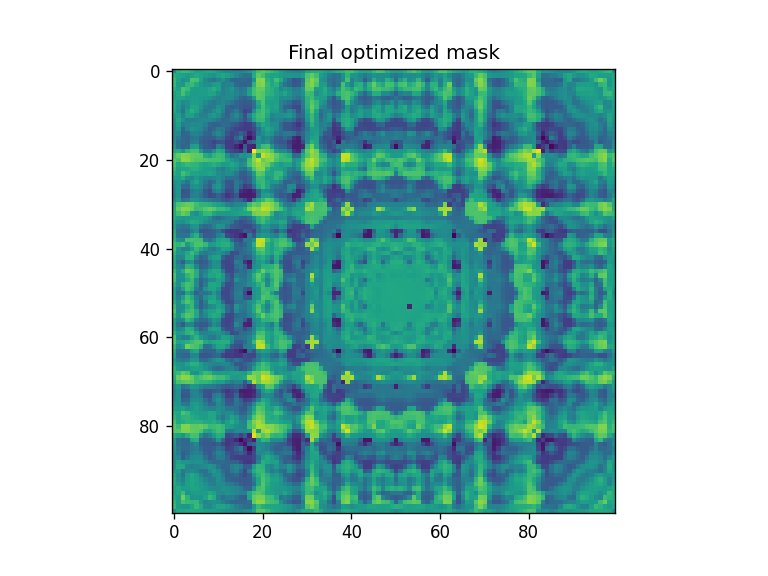
solution = moe.optimizer.optimize(logloss2, x0_flatten, args1=(aperture, screen, wavelength, target, "ASM", False), optimizer_method="dogbox", verbose=0, ftol=1e-5)

x = solution.x

fig = plt.figure()
xar = np.reshape(x, (x_pixel, y_pixel))
plt.imshow(xar)
plt.colorbar()
[42]:
<matplotlib.colorbar.Colorbar at 0x16da4fd7050>

[43]:
fig = plt.figure()
xar2 = np.reshape(x0_flatten, (x_pixel, y_pixel))
plt.imshow(xar2)
plt.title("Initial mask")
fig = plt.figure()
plt.imshow(np.abs(moe.optimizer.propagate(xar2, aperture, screen, wavelength) ) )
plt.title("Bluestein propagation from initial mask")
fig = plt.figure()
xar3 = np.reshape(x, (x_pixel, y_pixel))
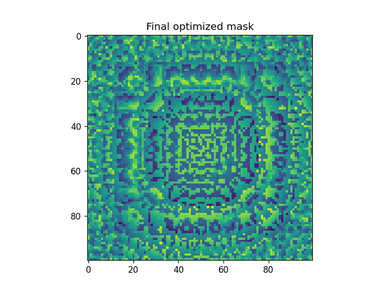
plt.imshow(xar3)
plt.title("Final optimized mask")
fig = plt.figure()
plt.imshow(np.abs(moe.optimizer.propagate(xar3, aperture, screen, wavelength) ) )
plt.title("Bluestein propagation from optimized mask")
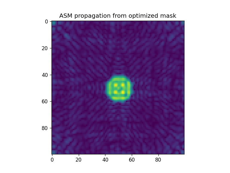
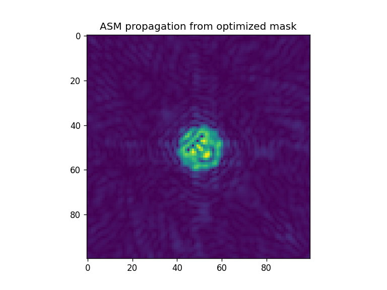
fig = plt.figure()
plt.imshow(np.abs(moe.optimizer.propagate(xar3, aperture, screen, wavelength, "ASM") ) )
plt.title("ASM propagation from optimized mask")
Elapsed: 0:00:00.017921
Elapsed: 0:00:00.013939
Elapsed: 0:00:00.014934
[43]:
Text(0.5, 1.0, 'ASM propagation from optimized mask')


[44]:
solution = moe.optimizer.optimize(logloss2, x0_flatten, args1=(aperture, screen, wavelength, target, "ASM", False), optimizer_method="dogbox", verbose=0, ftol=1e-3)

x = solution.x

fig = plt.figure()
xar = np.reshape(x, (x_pixel, y_pixel))
plt.imshow(xar)
plt.colorbar()
[44]:
<matplotlib.colorbar.Colorbar at 0x16dafff4cd0>
[45]:
loss_vector = solution.loss_history

plt.figure()
plt.plot(loss_vector)
plt.xlabel("Number iterations")
plt.ylabel("Loss (a.u.) ")
plt.tight_layout()
[46]:
#Uncomment to try any of these global optimization methods

##bounds = [(-np.pi, np.pi)]*len(x0_flatten)

#solution = moe.optimizer.optimize(logloss2, x0_flatten, args1=(aperture, screen,wavelength),  optimizer_method="dual_annealing", \
#                                  tol=1 , minimizer_kwargs={"args":(aperture, screen, wavelength), "tol": 1 },  bounds = bounds)

#solution = moe.optimizer.optimize(FOM2, x0_flatten, args1=(aperture, screen),  optimizer_method="basinhopping", tol=1 ,\
#                                  minimizer_kwargs={"args":(aperture, screen), "tol": 1 },  bounds = bounds)

#solution = moe.optimizer.optimize(FOM2, x0_flatten, args1=(aperture, screen),  optimizer_method="differential_evolution", tol=1 ,\
#                                  minimizer_kwargs={"args":(aperture, screen), "tol": 1 },  bounds = bounds)
Optimization with optax module optimizers
[47]:
solution = moe.optimizer.optimize(logloss2, x0_flatten, args1=(aperture, screen, wavelength, target, "ASM", False), \
                                  optimizer_method="adam", verbose=0, ftol=1e-5)
[48]:
x = solution.x

fig = plt.figure()
xar = np.reshape(x, (x_pixel, y_pixel))
plt.imshow(xar)
plt.colorbar()
[48]:
<matplotlib.colorbar.Colorbar at 0x16da532f950>
[49]:
fig = plt.figure()
xar2 = np.reshape(x0_flatten, (x_pixel, y_pixel))
plt.imshow(xar2)
plt.title("Initial mask")

fig = plt.figure()
plt.imshow(np.abs(moe.optimizer.propagate(xar2, aperture, screen, wavelength) ) )
plt.title("Bluestein propagation from initial mask")


fig = plt.figure()
xar3 = np.reshape(x, (x_pixel, y_pixel))
plt.imshow(xar3)
plt.title("Final optimized mask")

fig = plt.figure()
plt.imshow(np.abs(moe.optimizer.propagate(xar3, aperture, screen, wavelength) ) )
plt.title("Bluestein propagation from optimized mask")

fig = plt.figure()
plt.imshow(np.abs(moe.optimizer.propagate(xar3, aperture, screen, wavelength, "ASM") ) )
plt.title("ASM propagation from optimized mask")
Elapsed: 0:00:00.015930
Elapsed: 0:00:00.014935
Elapsed: 0:00:00.013939
[49]:
Text(0.5, 1.0, 'ASM propagation from optimized mask')


[50]:
loss_vector = solution.loss_history

plt.figure()
plt.plot(loss_vector)
plt.xlabel("Number iterations")
plt.ylabel("Loss (a.u.) ")
plt.tight_layout()
Bounds during optimization
By default the optimizers are unbound. Some can be bound, such as ‘dogbox’.
[51]:
## Optimization with bounds

solution = moe.optimizer.optimize(logloss2, x0_flatten, args1=(aperture, screen, wavelength, target, "bluestein", False), optimizer_method="dogbox", \
                                  bounds =(-1, 3), ftol = 1e-4 ,xtol=1e-12, )

x = solution.x

fig = plt.figure()
xar = np.reshape(x, (x_pixel, y_pixel))
plt.imshow(xar)
plt.colorbar()
`xtol` termination condition is satisfied.
Function evaluations 15, initial cost 3.9046e+01, final cost 1.4872e+01, first-order optimality 7.90e-04.
[51]:
<matplotlib.colorbar.Colorbar at 0x16d9d4bd550>
[52]:
fig = plt.figure()
xar3 = np.reshape(x, (x_pixel, y_pixel))
plt.imshow(xar3)
plt.title("Final optimized mask")

fig = plt.figure()
plt.imshow(np.abs(moe.optimizer.propagate(xar3, aperture, screen, wavelength) ) )
plt.title("Bluestein propagation from optimized mask")
Elapsed: 0:00:00.025887
[52]:
Text(0.5, 1.0, 'Bluestein propagation from optimized mask')
[53]:
loss_vector = solution.loss_history

plt.figure()
plt.plot(loss_vector)
plt.xlabel("Number iterations")
plt.ylabel("Loss (a.u.) ")
plt.tight_layout()
Hologram creation via inverse design
Binary hologram
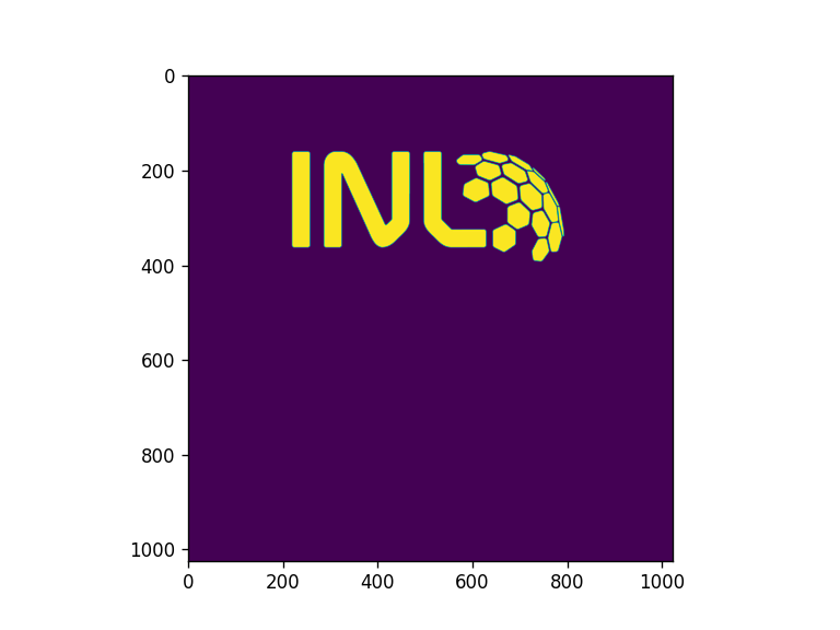
[54]:
file = "../5 - Holograms/target.png"
targetread = plt.imread(file)

x_pixel, y_pixel = np.shape(targetread)

xi = np.arange(x_pixel)
yi = np.arange(y_pixel)
XX, YY = np.meshgrid(xi,yi, indexing = 'ij')


fig = plt.figure()
plt.imshow(targetread)

targetread.shape
[54]:
(1024, 1024)
[55]:
fig = plt.figure()
plt.pcolormesh(XX,YY,targetread)
plt.gca().set_aspect('equal')
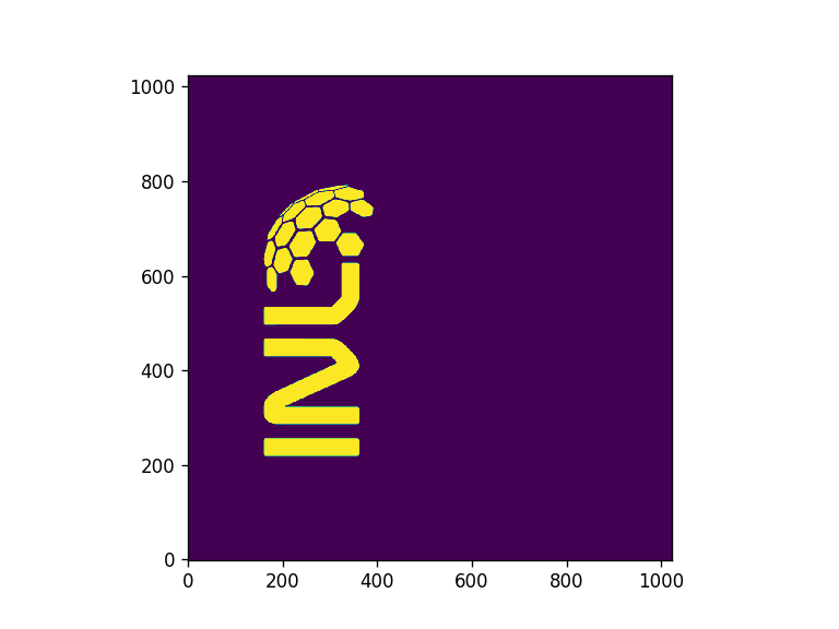
IMPORTANT the target is read as represented in the pcolormesh above in the ij indexing convention (used throughout the calculations). Hence, to have the correct representation, the axes need to be transformed.
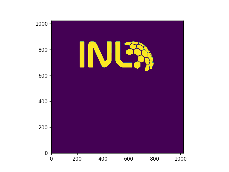
[56]:
target = np.flip(np.rot90(targetread))

#OR THIS ONE
#targetread = np.flipud(targetread)
#targetread = np.swapaxes(targetread, 0,1)

fig = plt.figure()
plt.pcolormesh(XX,YY,target)
plt.gca().set_aspect('equal')
[57]:
#Place holders for apertures

#size of the rectangular mask
aperture_width  = 50e-6 #m
aperture_height = 50e-6

pixsize = 1e-6 #m

wavelength = 500e-9 #m
focal_length = 200e-6

zmin = wavelength
zmax = 1.2* focal_length
nzs = 500

radius = aperture_width/2

# Create Aperture
aperture1 = moe.generate.create_empty_aperture(-aperture_width/2, aperture_width/2, x_pixel, -aperture_height/2, aperture_height/2, y_pixel)
[58]:
#Define Screen

# define the wavelength used in the propagation
wavelength = 532*nano

# Define the screen size and create it

screen_width = 2.5
screen_height = 2.5
x_pixel = 1024
y_pixel = 1024


# Creates a screen in YZ plane with [-aperture_height/2, aperture_height/2] and [zmin, zmax] and
ymin, ymax = -screen_height/2, screen_height/2
xmin, xmax = -screen_width/2, screen_width/2

s = 0.2

x = np.linspace(xmin*s, xmax*s, x_pixel)
y = np.linspace(ymin*s, ymax*s, y_pixel)
z = np.array([ s ])


screen = moe.Screen(x,y,z)
[59]:
# generation of initial guesses,

#random
xrand = np.random.rand(x_pixel, y_pixel)

plt.figure()
plt.imshow(xrand)

#constant
xvalues = np.ones((x_pixel, y_pixel))

plt.figure()
plt.imshow(xvalues)
#plt.colorbar()
[59]:
<matplotlib.image.AxesImage at 0x16da79ee6d0>
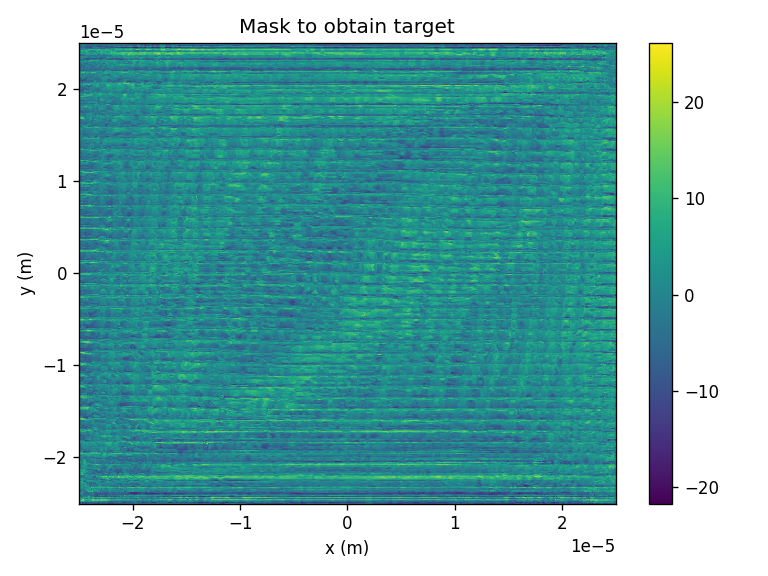
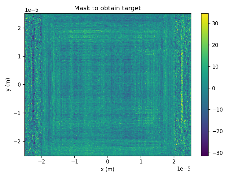
Binary hologram inverse design via MSE loss function
[60]:
def mselossmax(x, mask, screen, wavelength, target, use_timer=False, propag="bluestein", pad=2):
    import jax.numpy as jnp

    prop_x =  jnp.abs(moe.optimizer.propagate(jnp.reshape(x, (len(screen.x), len(screen.y))), mask, screen, wavelength,\
                                             propagation_method=propag, pad_factor=pad, use_timer=use_timer))**2

    diff = jnp.abs(prop_x/jnp.max(prop_x) - target/jnp.max(target))**2

    res = jnp.sum(diff)
    return res
[61]:
solution = moe.optimizer.optimize(mselossmax, x0= xvalues.flatten(), args1=[aperture1, screen, wavelength, target, False], verbose = 1, ftol=1e-6, xtol=None,\
                                  optimizer_method='dogbox', )


x2 = solution.x
`ftol` termination condition is satisfied.
Function evaluations 88, initial cost 1.8666e+09, final cost 3.8342e+08, first-order optimality 2.55e+03.
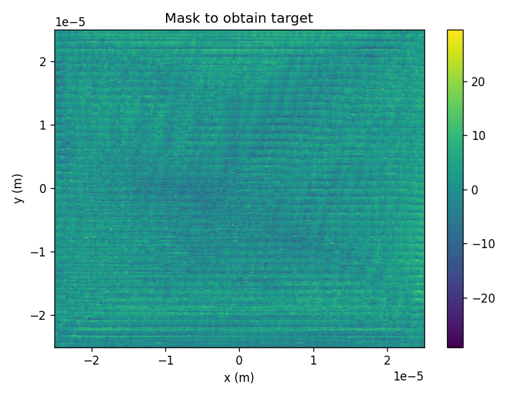
[62]:
xar3 = (np.reshape(x2, (x_pixel, y_pixel)))
# Create Aperture
aperture1 = moe.generate.create_empty_aperture(-aperture_width/2, aperture_width/2, x_pixel, -aperture_height/2, aperture_height/2, y_pixel)
fig = plt.figure()
plt.pcolormesh(aperture1.XX, aperture1.YY, xar3)
plt.title("Mask to obtain target")
plt.xlabel("x (m)")
plt.ylabel("y (m)")
plt.colorbar()
plt.tight_layout()
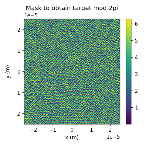
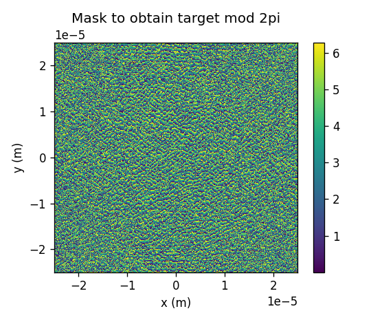
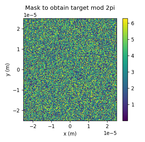
fig = plt.figure(figsize=(4.1,4))
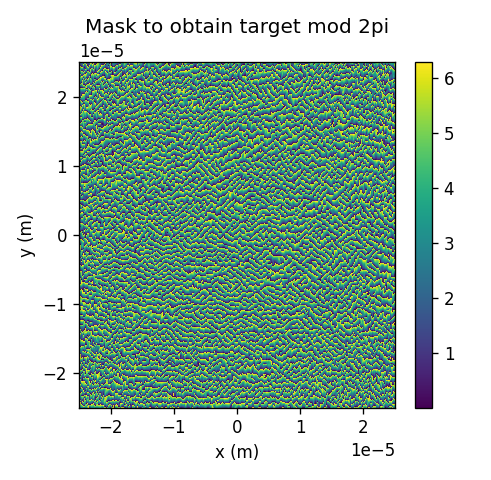
plt.pcolormesh(aperture1.XX, aperture1.YY, (xar3)%(2*np.pi) )
plt.title("Mask to obtain target mod 2pi")
plt.xlabel("x (m)")
plt.ylabel("y (m)")
plt.colorbar()
plt.tight_layout()
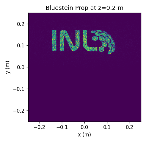
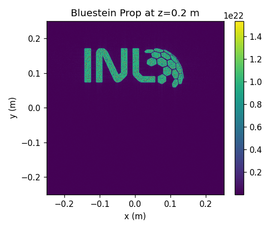
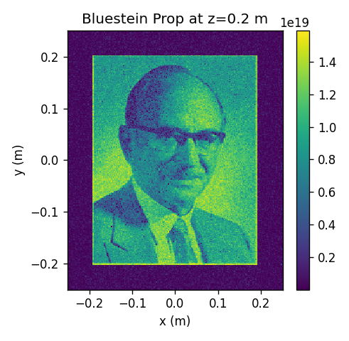
fig = plt.figure(figsize=(4.1,4))
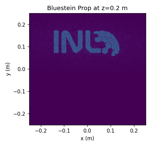
plt.pcolormesh(screen.XX[:,:,-1], screen.YY[:,:,-1], np.abs(moe.optimizer.propagate(xar3, aperture1, screen, wavelength) )**2 , vmax=5e22 )
plt.title("Bluestein Prop at z="+str(screen.z[-1])+" m")
plt.xlabel("x (m)")
plt.ylabel("y (m)")
plt.tight_layout()
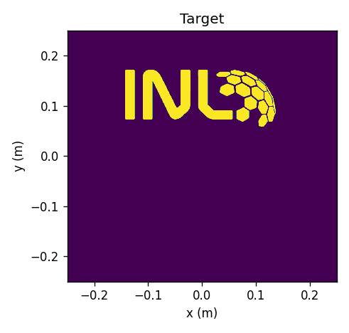
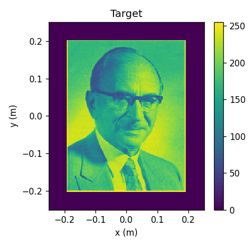
fig = plt.figure(figsize=(4.1,4))
plt.pcolormesh(screen.XX[:,:,-1], screen.YY[:,:,-1], (np.reshape(target, (x_pixel, y_pixel)) ))
plt.title("Target")
plt.xlabel("x (m)")
plt.ylabel("y (m)")
plt.tight_layout()
Elapsed: 0:00:00.607368

AGAIN, BEWARE all imshow will show rotated+flipped matrices, e.g. the optimization result shown below appers flipped and rotated!!!
[63]:
fig = plt.figure()
plt.pcolormesh((xar3) )
plt.colorbar()
plt.tight_layout()
[64]:
loss_vector = solution.loss_history

plt.figure()
plt.plot(loss_vector)
plt.xlabel("Number iterations")
plt.ylabel("Loss (a.u.) ")
plt.tight_layout()
Calculate the ISO uniformity of the inverse designed hologram.
[65]:
selection_mask = moe.generate.create_empty_aperture_from_aperture(aperture1)
selection_mask.aperture = target

moe.metrics.ISOuniformity(np.abs(moe.optimizer.propagate(xar3, aperture1, screen, wavelength)/1e5 )**2, selection_mask)
Elapsed: 0:00:00.597410
[65]:
0.5921155321872634
[66]:
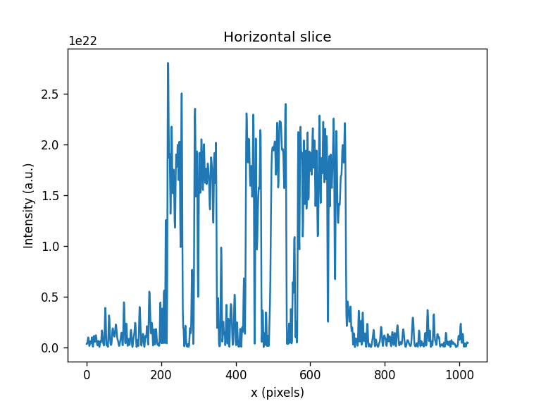
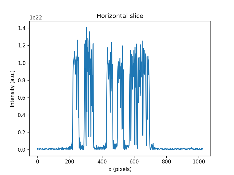
plt.figure()
prop = np.abs(moe.optimizer.propagate(xar3, aperture1, screen, wavelength) )**2
plt.plot(prop[:, 850])
plt.title("Horizontal slice")

plt.ylabel("Intensity (a.u.)")
plt.xlabel("x (pixels)")
Elapsed: 0:00:00.607359
[66]:
Text(0.5, 0, 'x (pixels)')
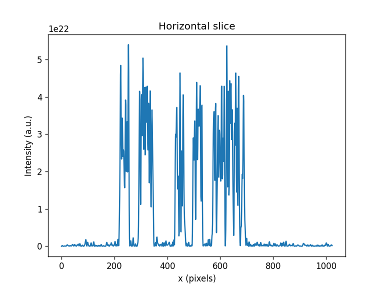
The horizontal slice and uniformity value demonstrate the hologram intensity it is not very uniform. We can calculate other metrics for information:
[67]:
it = np.abs(moe.optimizer.propagate(xar3, aperture1, screen, wavelength)/1e10 )**2


pwr = np.sum( it )
eff = moe.metrics.energy_eff(it, selection_mask)
snr = moe.metrics.snr(it, selection_mask)
npcc = moe.metrics.npcc(it, selection_mask.aperture)

pwr, eff, snr, npcc
Elapsed: 0:00:00.638201
[67]:
(17015624.0, 0.9117212, 44.23434257507324, 0.88908553)
[68]:
screen = moe.Screen(x,y,z)
# Define Aperture
aperture = moe.generate.create_empty_aperture(-aperture_width/2, aperture_width/2, x_pixel, -aperture_height/2, aperture_height/2, y_pixel)
mask_amplitude = moe.generate.create_empty_aperture_from_aperture(aperture)
# Define Phase mask
mask_phase = moe.generate.create_empty_aperture_from_aperture(aperture)
mask_phase.aperture = xar3
#mask_phase.aperture = np.flipud(np.rot90(xar3)) ##use need to
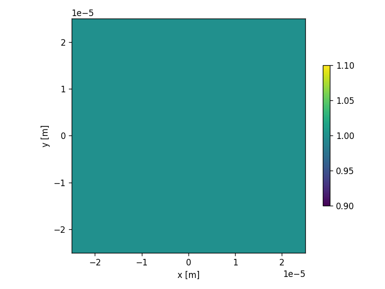
mask_amplitude.aperture = mask_amplitude.aperture +1
# Plot the circular mask
moe.plotting.plot_aperture(mask_phase)
moe.plotting.plot_aperture(mask_amplitude)
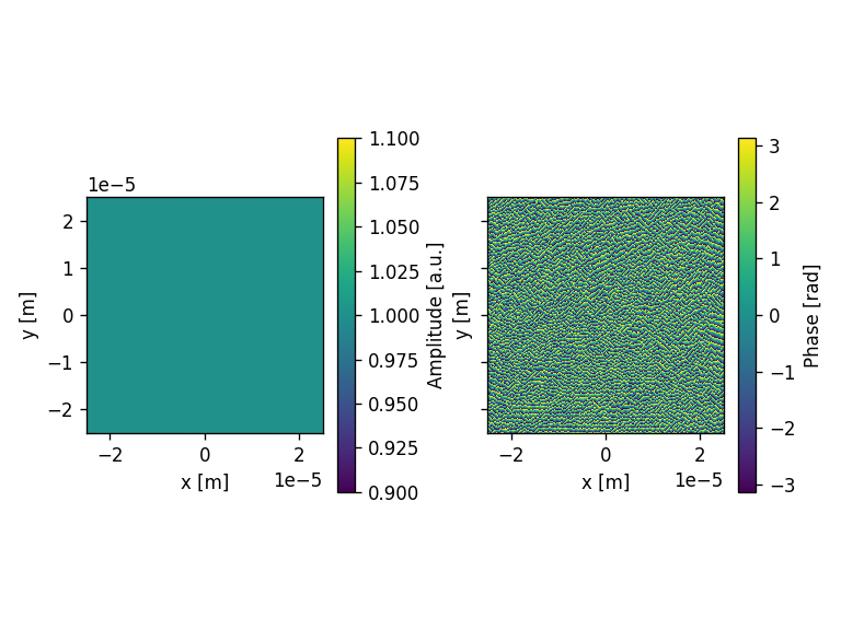
# Calculates a field to use with the calculated mask
# Initialize a Field from the Aperture mask
field = moe.field.create_empty_field_from_aperture(mask_phase)
# Generate a uniform field
field = moe.field.generate_uniform_field(field, E0=1)
# Modulates the field with a given aperture that can be used either as an amplitude mask or a phase mask
field = moe.field.modulate_field(field, amplitude_mask=mask_amplitude, phase_mask=mask_phase)
# Plots the field (amplitude and phase)
moe.plotting.plot_field(field)
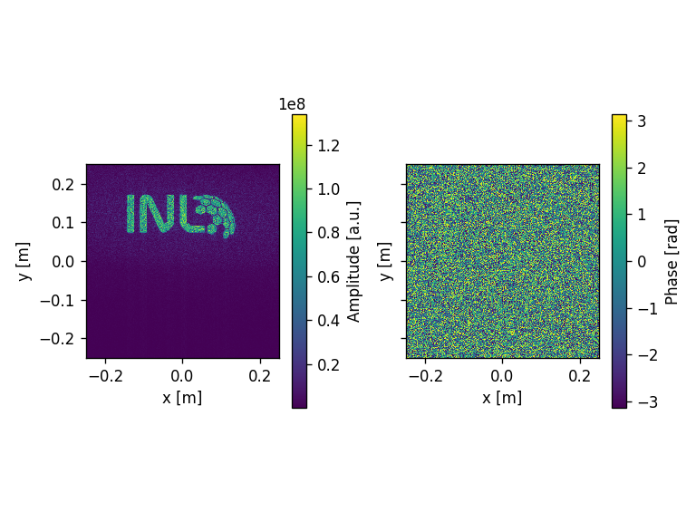
# Propagate the field with Bluestein
EXYZ = moe.propagate.Bluestein(field, screen, wavelength)
moe.plotting.plot_screen_XY(EXYZ, z=s)
Progress: [####################] 100.0%
Elapsed: 0:00:01.063358
Improving uniformity for the binary hologram inverse design via loss function engineering
[69]:
def lossunif(x, mask, screen, wavelength, target, selection_mask, use_timer=False, propag="bluestein", pad=2):
    import jax.numpy as jnp
    import jax

    prop_x =  jnp.abs(moe.optimizer.propagate(jnp.reshape(x, (len(screen.x), len(screen.y))), mask, screen, wavelength,\
                                             propagation_method=propag, pad_factor=pad, use_timer=use_timer)/1e10)**2

    unif =  moe.metrics.ISOuniformity(prop_x, selection_mask, optimize=True)

    res = unif

    jax.debug.print("{}",res)

    return res


selection_mask = moe.generate.create_empty_aperture_from_aperture(aperture1)

selection_mask.aperture = target

solution = moe.optimizer.optimize(lossunif,  x0= x2, args1=[aperture, screen, wavelength, target, selection_mask, False], \
                                  verbose = 1, ftol=1e-2, xtol=None, optimizer_method='dogbox', )

x = solution.x
0.5921157002449036
0.5921157002449036
0.5921157002449036
0.9359090328216553
0.9359090328216553
0.5459924936294556
0.5459924936294556
0.5459924936294556
0.56988126039505
0.56988126039505
0.5105724930763245
0.5105724930763245
0.5105724930763245
0.49339035153388977
0.49339035153388977
0.49339035153388977
0.4698822796344757
0.4698822796344757
0.4698822796344757
0.44474607706069946
0.44474607706069946
0.44474607706069946
0.528486430644989
0.528486430644989
0.4298486113548279
0.4298486113548279
0.4298486113548279
0.42245784401893616
0.42245784401893616
0.42245784401893616
0.4163167476654053
0.4163167476654053
0.4163167476654053
0.41169631481170654
0.41169631481170654
0.41169631481170654
0.4065950810909271
0.4065950810909271
0.4065950810909271
0.40148162841796875
0.40148162841796875
0.40148162841796875
0.3982401490211487
0.3982401490211487
0.3982401490211487
0.39462241530418396
0.39462241530418396
0.39462241530418396
0.390697181224823
0.390697181224823
0.390697181224823
0.3871155083179474
0.3871155083179474
0.3871155083179474
0.3837389349937439
0.3837389349937439
0.3837389349937439
0.38086801767349243
0.38086801767349243
0.38086801767349243
0.3782268166542053
0.3782268166542053
0.3782268166542053
0.3758487105369568
0.3758487105369568
0.3758487105369568
0.37363681197166443
0.37363681197166443
0.37363681197166443
0.37154147028923035
0.37154147028923035
0.37154147028923035
0.3696393668651581
0.3696393668651581
0.3696393668651581
0.3677220940589905
0.3677220940589905
0.3677220940589905
0.3660847842693329
0.3660847842693329
0.3660847842693329
`ftol` termination condition is satisfied.
Function evaluations 28, initial cost 1.7530e-01, final cost 6.7009e-02, first-order optimality 5.31e-07.
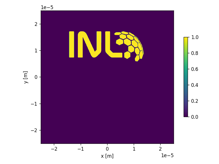
[70]:
selection_mask.aperture = target

moe.plotting.plot_aperture(selection_mask)
[71]:
xar3 = (np.reshape(x, (x_pixel, y_pixel)))
# Create Aperture
aperture1 = moe.generate.create_empty_aperture(-aperture_width/2, aperture_width/2, x_pixel, -aperture_height/2, aperture_height/2, y_pixel)
fig = plt.figure()
plt.pcolormesh(aperture1.XX, aperture1.YY, xar3)
plt.title("Mask to obtain target")
plt.xlabel("x (m)")
plt.ylabel("y (m)")
plt.colorbar()
plt.tight_layout()
fig = plt.figure(figsize=(4.1,4))
plt.pcolormesh(aperture1.XX, aperture1.YY, (xar3)%(2*np.pi) )
plt.title("Mask to obtain target mod 2pi")
plt.xlabel("x (m)")
plt.ylabel("y (m)")
plt.colorbar()
plt.tight_layout()
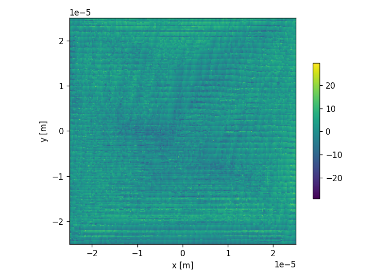
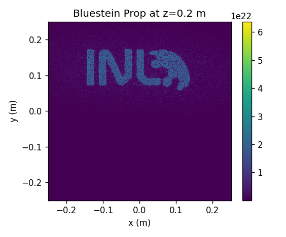
fig = plt.figure(figsize=(4.1,4))
plt.pcolormesh(screen.XX[:,:,-1], screen.YY[:,:,-1], np.abs(moe.optimizer.propagate(xar3, aperture1, screen, wavelength) )**2 )
plt.title("Bluestein Prop at z="+str(screen.z[-1])+" m")
plt.xlabel("x (m)")
plt.ylabel("y (m)")
plt.tight_layout()
fig = plt.figure(figsize=(4.1,4))
plt.pcolormesh(screen.XX[:,:,-1], screen.YY[:,:,-1], (np.reshape(target, (x_pixel, y_pixel)) ))
plt.title("Target")
plt.xlabel("x (m)")
plt.ylabel("y (m)")
plt.tight_layout()
Elapsed: 0:00:00.596075


[72]:
plt.figure()
prop = np.abs(moe.optimizer.propagate(xar3, aperture1, screen, wavelength) )**2
plt.plot(prop[:, 850])

plt.title("Horizontal slice")

plt.ylabel("Intensity (a.u.)")
plt.xlabel("x (pixels)")
Elapsed: 0:00:00.545605
[72]:
Text(0.5, 0, 'x (pixels)')
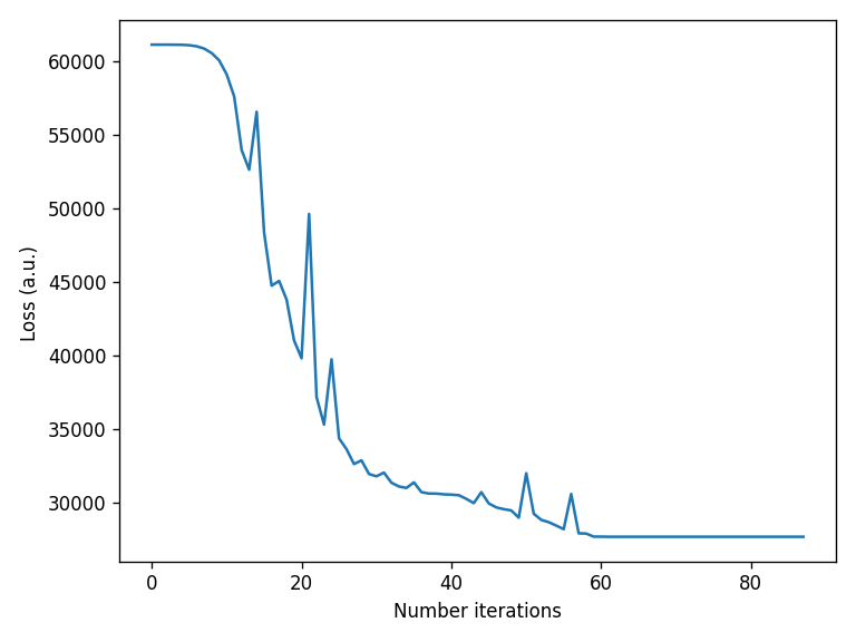
[73]:
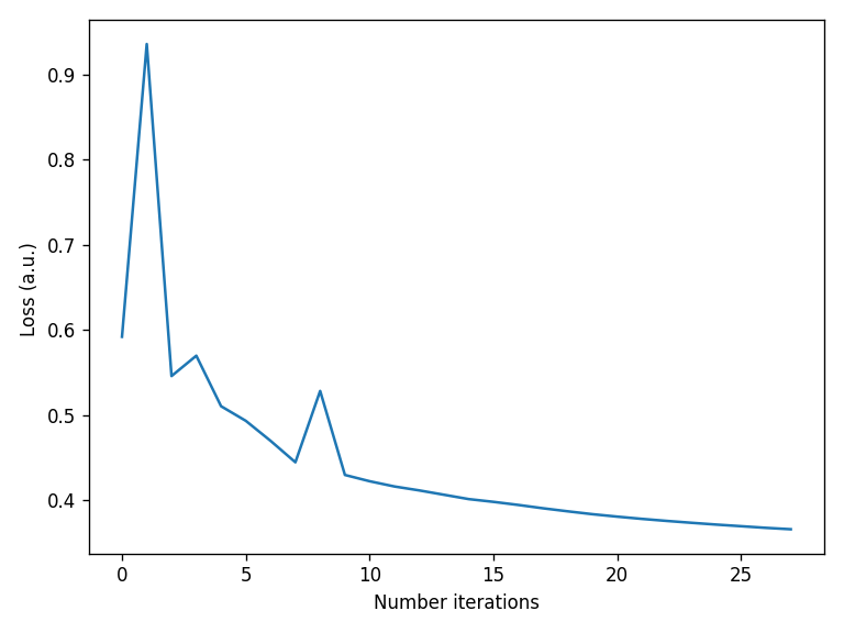
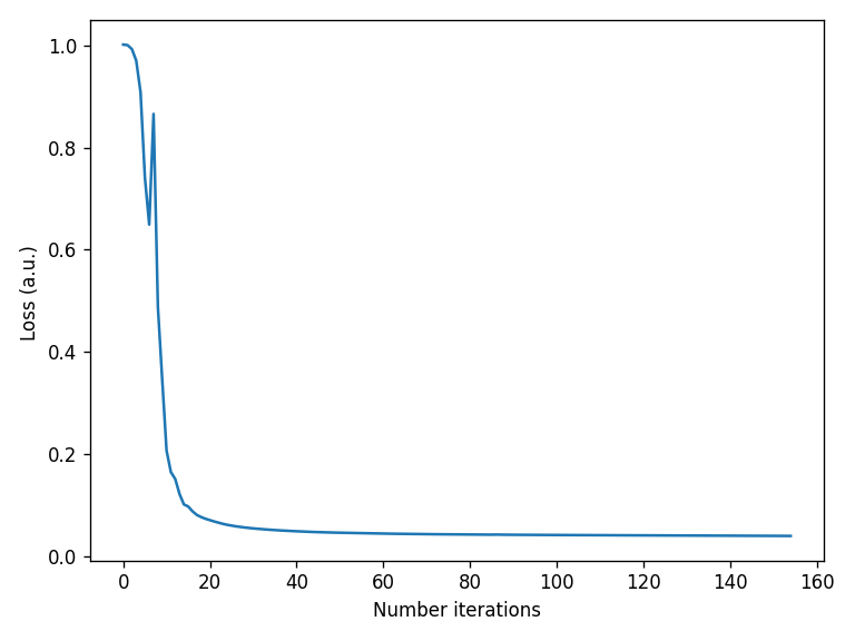
loss_vector = solution.loss_history

plt.figure()
plt.plot(loss_vector)
plt.xlabel("Number iterations")
plt.ylabel("Loss (a.u.) ")
plt.tight_layout()
[74]:
selection_mask = moe.generate.create_empty_aperture_from_aperture(aperture1)
selection_mask.aperture = target

moe.metrics.ISOuniformity(np.abs(moe.optimizer.propagate(xar3, aperture1, screen, wavelength)/1e5 )**2, selection_mask)
Elapsed: 0:00:00.543171
[74]:
0.3660847310490504
[75]:
it = np.abs(moe.optimizer.propagate(xar3, aperture1, screen, wavelength)/1e10 )**2


pwr = np.sum( it )
eff = moe.metrics.energy_eff(it, selection_mask)
snr = moe.metrics.snr(it, selection_mask)
npcc = moe.metrics.npcc(it, selection_mask.aperture)

pwr, eff, snr, npcc
Elapsed: 0:00:00.546599
[75]:
(15793504.0, 0.6519183, 29.404501914978027, 0.8890994)
Binary hologram inverse design via Negative Peason Correlation Coefficient (NPCC) loss function
[76]:
def npccloss(x, mask, screen, wavelength, target, selection_mask, use_timer=False, propag="bluestein", pad=2):
    import jax.numpy as jnp

    prop_x =  jnp.abs(moe.optimizer.propagate(jnp.reshape(x, (len(screen.x), len(screen.y))), mask, screen, wavelength,\
                                             propagation_method=propag, pad_factor=pad, use_timer=use_timer)/1e10)**2

    npcc =  (moe.metrics.npcc(prop_x, target, optimize=True) )

    res = 1 - npcc

    #print(npcc)

    return res


solution = moe.optimizer.optimize(npccloss, x0= xvalues.flatten(), args1=[aperture1, screen, wavelength, target, False], verbose = 1, \
                                  ftol=1e-3, xtol=None,\
                                  optimizer_method='trf', )

x = solution.x
`ftol` termination condition is satisfied.
Function evaluations 155, initial cost 5.0160e-01, final cost 7.8925e-04, first-order optimality 8.34e-09.
[77]:
xar3 = (np.reshape(x, (x_pixel, y_pixel)))

# Create Aperture
aperture1 = moe.generate.create_empty_aperture(-aperture_width/2, aperture_width/2, x_pixel, -aperture_height/2, aperture_height/2, y_pixel)

fig = plt.figure()

plt.pcolormesh(aperture1.XX, aperture1.YY, xar3)
plt.title("Mask to obtain target")
plt.xlabel("x (m)")
plt.ylabel("y (m)")
plt.colorbar()
plt.tight_layout()

fig = plt.figure(figsize=(4.5,3.9))
plt.pcolormesh(aperture1.XX, aperture1.YY, (xar3)%(2*np.pi) )
plt.title("Mask to obtain target mod 2pi")
plt.xlabel("x (m)")
plt.ylabel("y (m)")
plt.colorbar()
plt.tight_layout()

fig = plt.figure(figsize=(4.7,3.9))
plt.pcolormesh(screen.XX[:,:,-1], screen.YY[:,:,-1], np.abs(moe.optimizer.propagate(xar3, aperture1, screen, wavelength) )**2 )
plt.title("Bluestein Prop at z="+str(screen.z[-1])+" m")
plt.xlabel("x (m)")
plt.ylabel("y (m)")
plt.colorbar()
plt.tight_layout()

fig = plt.figure(figsize=(4.1,3.9))
plt.pcolormesh(screen.XX[:,:,-1], screen.YY[:,:,-1], (np.reshape(target, (x_pixel, y_pixel)) ))
plt.title("Target")
plt.xlabel("x (m)")
plt.ylabel("y (m)")
plt.tight_layout()
Elapsed: 0:00:00.569498
[78]:
plt.figure()
prop = np.abs(moe.optimizer.propagate(xar3, aperture1, screen, wavelength) )**2
plt.plot(prop[:, 850])
plt.title("Horizontal slice")

plt.ylabel("Intensity (a.u.)")
plt.xlabel("x (pixels)")
Elapsed: 0:00:00.554601
[78]:
Text(0.5, 0, 'x (pixels)')
[79]:
loss_vector = solution.loss_history

plt.figure()
plt.plot(loss_vector)
plt.xlabel("Number iterations")
plt.ylabel("Loss (a.u.) ")
plt.tight_layout()
[80]:
selection_mask = moe.generate.create_empty_aperture_from_aperture(aperture1)
selection_mask.aperture = target

moe.metrics.ISOuniformity(np.abs(moe.optimizer.propagate(xar3, aperture1, screen, wavelength)/1e5 )**2, selection_mask)
Elapsed: 0:00:00.574502
[80]:
0.3810365200699862
[81]:
it = np.abs(moe.optimizer.propagate(xar3, aperture1, screen, wavelength)/1e10 )**2


pwr = np.sum( it )
eff = moe.metrics.energy_eff(it, selection_mask)
snr = moe.metrics.snr(it, selection_mask)
npcc = moe.metrics.npcc(it, target)

pwr, eff, snr, npcc
Elapsed: 0:00:00.605395
[81]:
(6441096.0, 0.8515422, 39.12632465362549, 0.96026903)
[82]:
def lossunif(x, mask, screen, wavelength, target, selection_mask, use_timer=False, propag="bluestein", pad=2):
    import jax.numpy as jnp
    import jax

    prop_x =  jnp.abs(moe.optimizer.propagate(jnp.reshape(x, (len(screen.x), len(screen.y))), mask, screen, wavelength,\
                                             propagation_method=propag, pad_factor=pad, use_timer=use_timer)/1e10)**2

    unif =  moe.metrics.ISOuniformity(prop_x, selection_mask, optimize=True)

    res = unif

    jax.debug.print("{}",res)

    return res


selection_mask = moe.generate.create_empty_aperture_from_aperture(aperture1)

selection_mask.aperture = target


solution = moe.optimizer.optimize(lossunif,  x0= x2, args1=[aperture, screen, wavelength, target, selection_mask, False], \
                                  verbose = 1, ftol=1e-2, xtol=None, optimizer_method='dogbox', )

x = solution.x
0.5921157002449036
0.5921157002449036
0.5921157002449036
0.9359090328216553
0.9359090328216553
0.5459924936294556
0.5459924936294556
0.5459924936294556
0.56988126039505
0.56988126039505
0.5105724930763245
0.5105724930763245
0.5105724930763245
0.49339035153388977
0.49339035153388977
0.49339035153388977
0.4698822796344757
0.4698822796344757
0.4698822796344757
0.44474607706069946
0.44474607706069946
0.44474607706069946
0.528486430644989
0.528486430644989
0.4298486113548279
0.4298486113548279
0.4298486113548279
0.42245784401893616
0.42245784401893616
0.42245784401893616
0.4163167476654053
0.4163167476654053
0.4163167476654053
0.41169631481170654
0.41169631481170654
0.41169631481170654
0.4065950810909271
0.4065950810909271
0.4065950810909271
0.40148162841796875
0.40148162841796875
0.40148162841796875
0.3982401490211487
0.3982401490211487
0.3982401490211487
0.39462241530418396
0.39462241530418396
0.39462241530418396
0.390697181224823
0.390697181224823
0.390697181224823
0.3871155083179474
0.3871155083179474
0.3871155083179474
0.3837389349937439
0.3837389349937439
0.3837389349937439
0.38086801767349243
0.38086801767349243
0.38086801767349243
0.3782268166542053
0.3782268166542053
0.3782268166542053
0.3758487105369568
0.3758487105369568
0.3758487105369568
0.37363681197166443
0.37363681197166443
0.37363681197166443
0.37154147028923035
0.37154147028923035
0.37154147028923035
0.3696393668651581
0.3696393668651581
0.3696393668651581
0.3677220940589905
0.3677220940589905
0.3677220940589905
0.3660847842693329
0.3660847842693329
0.3660847842693329
`ftol` termination condition is satisfied.
Function evaluations 28, initial cost 1.7530e-01, final cost 6.7009e-02, first-order optimality 5.31e-07.
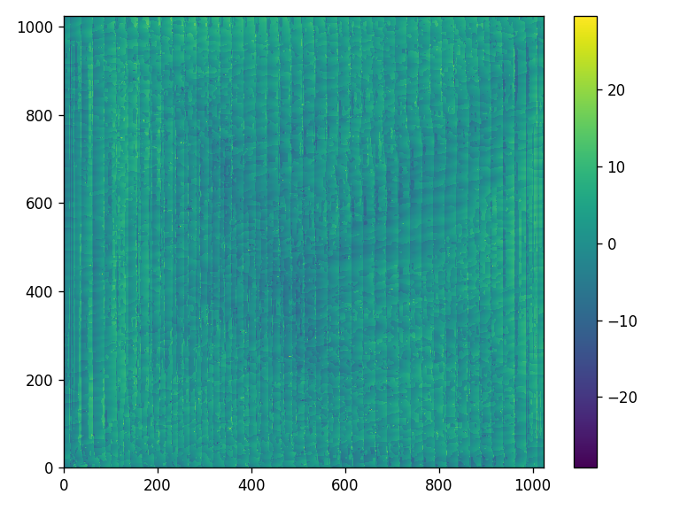
[83]:
xar3 = (np.reshape(x, (x_pixel, y_pixel)))

# Create Aperture
aperture1 = moe.generate.create_empty_aperture(-aperture_width/2, aperture_width/2, x_pixel, -aperture_height/2, aperture_height/2, y_pixel)

fig = plt.figure()

plt.pcolormesh(aperture1.XX, aperture1.YY, xar3)
plt.title("Mask to obtain target")
plt.xlabel("x (m)")
plt.ylabel("y (m)")
plt.colorbar()
plt.tight_layout()

fig = plt.figure(figsize=(4.5,3.9))
plt.pcolormesh(aperture1.XX, aperture1.YY, (xar3)%(2*np.pi) )
plt.title("Mask to obtain target mod 2pi")
plt.xlabel("x (m)")
plt.ylabel("y (m)")
plt.colorbar()
plt.tight_layout()

fig = plt.figure(figsize=(4.7,3.9))
plt.pcolormesh(screen.XX[:,:,-1], screen.YY[:,:,-1], np.abs(moe.optimizer.propagate(xar3, aperture1, screen, wavelength) )**2 )
plt.title("Bluestein Prop at z="+str(screen.z[-1])+" m")
plt.xlabel("x (m)")
plt.ylabel("y (m)")
plt.colorbar()
plt.tight_layout()

fig = plt.figure(figsize=(4.1,3.9))
plt.pcolormesh(screen.XX[:,:,-1], screen.YY[:,:,-1], (np.reshape(target, (x_pixel, y_pixel)) ))
plt.title("Target")
plt.xlabel("x (m)")
plt.ylabel("y (m)")
plt.tight_layout()

plt.figure()
prop = np.abs(moe.optimizer.propagate(xar3, aperture1, screen, wavelength) )**2
plt.plot(prop[:, 850])
plt.title("Horizontal slice")

plt.ylabel("Intensity (a.u.)")
plt.xlabel("x (pixels)")
Elapsed: 0:00:00.619332
Elapsed: 0:00:00.546605
[83]:
Text(0.5, 0, 'x (pixels)')


[84]:
it = np.abs(moe.optimizer.propagate(xar3, aperture1, screen, wavelength)/1e10 )**2

#Metrics
pwr = np.sum( it )
eff = moe.metrics.energy_eff(it, selection_mask)
snr = moe.metrics.snr(it, selection_mask)
npcc = moe.metrics.npcc(it, selection_mask.aperture)

pwr, eff, snr, npcc
Elapsed: 0:00:00.588403
[84]:
(15793504.0, 0.6519183, 29.404501914978027, 0.8890994)
Grayscale hologram
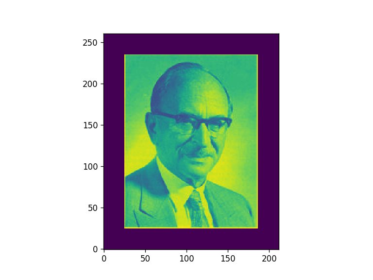
[85]:
file = "../5 - Holograms/Gabor.jpg"
targetread = plt.imread(file)

targetread = targetread[:,:,0]
targetread = np.flip(np.rot90(targetread))

targetread = np.pad(targetread, 25)
[86]:
x_pixel, y_pixel = np.shape(targetread)

xi = np.arange(x_pixel)
yi = np.arange(y_pixel)
XX, YY = np.meshgrid(xi,yi, indexing = 'ij')


fig = plt.figure()
plt.pcolormesh(XX,YY,targetread)
plt.gca().set_aspect('equal')
[87]:
target = targetread


#size of the rectangular mask
aperture_width  = 50e-6 #m
aperture_height = 50e-6

pixsize = 1e-6 #m

wavelength = 500e-9 #m
focal_length = 200e-6

zmin = wavelength
zmax = 1.2* focal_length
nzs = 500

radius = aperture_width/2

# Create Aperture
aperture1 = moe.generate.create_empty_aperture(-aperture_width/2, aperture_width/2, x_pixel, -aperture_height/2, aperture_height/2, y_pixel)


#Define Screen

# define the wavelength used in the propagation
wavelength = 532*nano

# Define the screen size and create it

screen_width = 2.5
screen_height = 2.5


# Creates a screen in YZ plane with [-aperture_height/2, aperture_height/2] and [zmin, zmax] and
ymin, ymax = -screen_height/2, screen_height/2
xmin, xmax = -screen_width/2, screen_width/2

s = 0.2

x = np.linspace(xmin*s, xmax*s, x_pixel)
y = np.linspace(ymin*s, ymax*s, y_pixel)
z = np.array([ s ])


screen = moe.Screen(x,y,z)

# generation of initial guesses,

#random
xrand = np.random.rand(x_pixel, y_pixel)


#constant
xvalues = np.ones((x_pixel, y_pixel))
Grayscale hologram generation with MSE loss function
[88]:
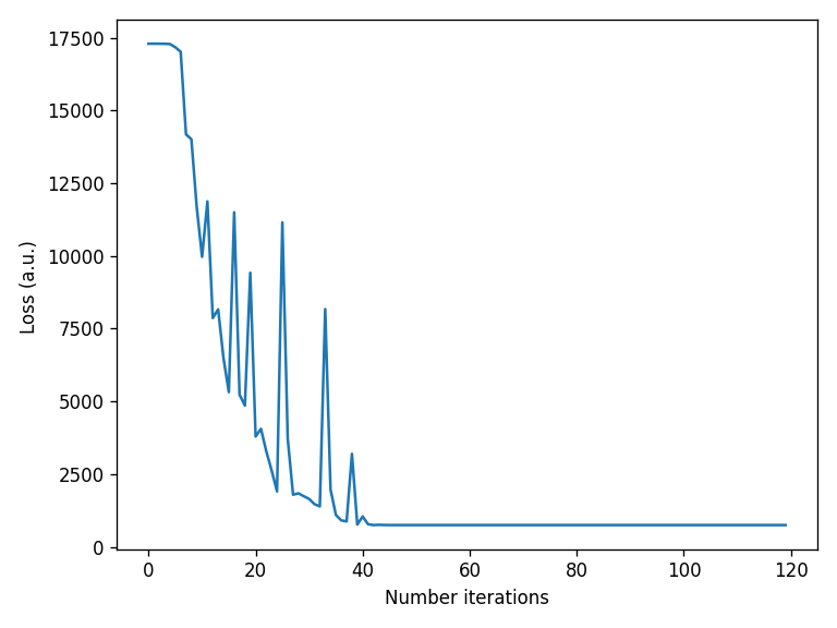
solution = moe.optimizer.optimize(mselossmax, x0= xvalues.flatten(), args1=[aperture1, screen, wavelength, target, False], verbose = 1, ftol=1e-8, xtol=None,\
                                  optimizer_method='dogbox', )


x2 = solution.x
`ftol` termination condition is satisfied.
Function evaluations 120, initial cost 1.4964e+08, final cost 2.7909e+05, first-order optimality 8.42e+01.
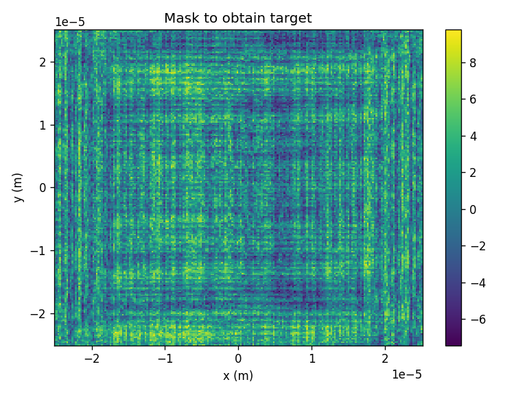
[89]:
xar3 = (np.reshape(x2, (x_pixel, y_pixel)))
# Create Aperture
aperture1 = moe.generate.create_empty_aperture(-aperture_width/2, aperture_width/2, x_pixel, -aperture_height/2, aperture_height/2, y_pixel)
fig = plt.figure()
plt.pcolormesh(aperture1.XX, aperture1.YY, xar3)
plt.title("Mask to obtain target")
plt.xlabel("x (m)")
plt.ylabel("y (m)")
plt.colorbar()
plt.tight_layout()
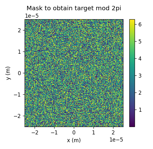
fig = plt.figure(figsize=(4.1,4))
plt.pcolormesh(aperture1.XX, aperture1.YY, (xar3)%(2*np.pi) )
plt.title("Mask to obtain target mod 2pi")
plt.xlabel("x (m)")
plt.ylabel("y (m)")
plt.colorbar()
plt.tight_layout()
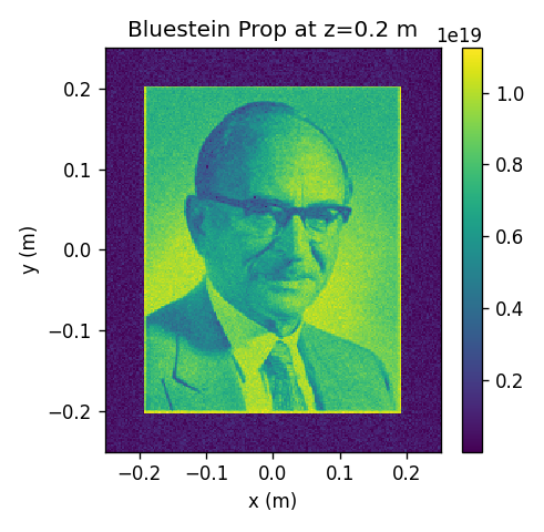
fig = plt.figure(figsize=(4.1,4))
plt.pcolormesh(screen.XX[:,:,-1], screen.YY[:,:,-1], np.abs(moe.optimizer.propagate(xar3, aperture1, screen, wavelength) )**2 )
plt.title("Bluestein Prop at z="+str(screen.z[-1])+" m")
plt.xlabel("x (m)")
plt.ylabel("y (m)")
plt.tight_layout()
plt.colorbar()
fig = plt.figure(figsize=(4.1,4))
plt.pcolormesh(screen.XX[:,:,-1], screen.YY[:,:,-1], (np.reshape(target, (x_pixel, y_pixel)) ))
plt.title("Target")
plt.xlabel("x (m)")
plt.ylabel("y (m)")
plt.tight_layout()
plt.colorbar()
loss_vector = solution.loss_history
plt.figure()
plt.plot(loss_vector)
plt.xlabel("Number iterations")
plt.ylabel("Loss (a.u.) ")
plt.tight_layout()
Elapsed: 0:00:00.049844
[90]:
moe.metrics.npcc(np.abs(moe.optimizer.propagate(xar3, aperture1, screen, wavelength) /1e10)**2, target)
Elapsed: 0:00:00.044803
[90]:
0.9769124124498108
Grayscale hologram generation with NPCC loss function
[91]:
def npccloss(x, mask, screen, wavelength, target, selection_mask, use_timer=False, propag="bluestein", pad=2):
    import jax.numpy as jnp

    prop_x =  jnp.abs(moe.optimizer.propagate(jnp.reshape(x, (len(screen.x), len(screen.y))), mask, screen, wavelength,\
                                             propagation_method=propag, pad_factor=pad, use_timer=use_timer)/1e10)**2

    npcc =  jnp.abs(moe.metrics.npcc(prop_x, target, optimize=True) )

    res = 1 - npcc

    #print(npcc)

    return res


solution = moe.optimizer.optimize(npccloss, x0= xvalues.flatten(), args1=[aperture1, screen, wavelength, target, False], verbose = 1, ftol=1e-12, xtol=None,\
                                  optimizer_method='adamw', )

x = solution.x
[92]:
xar3 = (np.reshape(x, (x_pixel, y_pixel)))

# Create Aperture
aperture1 = moe.generate.create_empty_aperture(-aperture_width/2, aperture_width/2, x_pixel, -aperture_height/2, aperture_height/2, y_pixel)

fig = plt.figure()

plt.pcolormesh(aperture1.XX, aperture1.YY, xar3)
plt.title("Mask to obtain target")
plt.xlabel("x (m)")
plt.ylabel("y (m)")
plt.colorbar()
plt.tight_layout()

fig = plt.figure(figsize=(4.1,4))
plt.pcolormesh(aperture1.XX, aperture1.YY, (xar3)%(2*np.pi) )
plt.title("Mask to obtain target mod 2pi")
plt.xlabel("x (m)")
plt.ylabel("y (m)")
plt.colorbar()
plt.tight_layout()

fig = plt.figure(figsize=(4.1,4))
plt.pcolormesh(screen.XX[:,:,-1], screen.YY[:,:,-1], np.abs(moe.optimizer.propagate(xar3, aperture1, screen, wavelength) )**2 )
plt.title("Bluestein Prop at z="+str(screen.z[-1])+" m")
plt.xlabel("x (m)")
plt.ylabel("y (m)")
plt.tight_layout()
plt.colorbar()

fig = plt.figure(figsize=(4.1,4))
plt.pcolormesh(screen.XX[:,:,-1], screen.YY[:,:,-1], (np.reshape(target, (x_pixel, y_pixel)) ))
plt.title("Target")
plt.xlabel("x (m)")
plt.ylabel("y (m)")
plt.tight_layout()
plt.colorbar()


loss_vector = solution.loss_history

plt.figure()
plt.plot(loss_vector)
plt.xlabel("Number iterations")
plt.ylabel("Loss (a.u.) ")
plt.tight_layout()
Elapsed: 0:00:00.053762

[93]:
moe.metrics.npcc(np.abs(moe.optimizer.propagate(xar3, aperture1, screen, wavelength) /1e10)**2, target)
Elapsed: 0:00:00.044844
[93]:
0.9955662758957005
Optimization of ensembles of optical elements
[94]:
###Import two surfaces - doublet

#number of pixels
x_pixel = 100
y_pixel = 100

a1_phase = np.random.rand(x_pixel, y_pixel) #np.genfromtxt("asph1_phase.csv", delimiter=',')
a1_inten = a1_phase * 0 #np.genfromtxt("asph1_inten.csv", delimiter=',')

a2_phase = np.random.rand(x_pixel, y_pixel) #np.genfromtxt("asph2_phase.csv", delimiter=',')
a2_inten = a2_phase * 0 #np.genfromtxt("asph2_inten.csv", delimiter=',')


#size of the rectangular mask
aperture_width  = 800e-6 #m
aperture_height = 800e-6

pixsize = 8e-6 #m

wavelength = 550e-9

dist1 = 40e-3
dist2 = 50e-3

zmin1 = wavelength
zmax1 = dist1
nzs = 2

zmin2 = wavelength
zmax2 = dist2
nzs = 2

radius = aperture_width/2


asph1_mask_phase = moe.generate.create_empty_aperture(-aperture_width/2, aperture_width/2, x_pixel, -aperture_height/2, aperture_height/2, y_pixel)
asph1_mask_phase.aperture = a1_phase

asph1_mask_inten = moe.generate.create_empty_aperture_from_aperture(asph1_mask_phase)
asph1_mask_inten.aperture = a1_inten

asph2_mask_phase = moe.generate.create_empty_aperture(-aperture_width/2, aperture_width/2, x_pixel, -aperture_height/2, aperture_height/2, y_pixel)
asph2_mask_phase.aperture = a2_phase

asph2_mask_inten = moe.generate.create_empty_aperture_from_aperture(asph2_mask_phase)
asph2_mask_inten.aperture = a2_inten

aperture = moe.generate.create_empty_aperture_from_aperture(asph2_mask_phase)
mask = moe.generate.circular_aperture(aperture, radius=radius*10)

aperture_array_phase = [asph1_mask_phase, asph2_mask_phase]
aperture_array_amp = [mask,]*len(aperture_array_phase)

############################
## Define the screens
x1 = asph1_mask_phase.x
y1 = asph1_mask_phase.y
z1 = np.linspace(zmin1, zmax1, nzs)

screen1 = moe.field.Screen(x1,y1,z1)

x2 = asph2_mask_phase.x
y2 = asph2_mask_phase.y
z2 = np.linspace(zmin2, zmax2, nzs)

screen2 = moe.field.Screen(x2,y2,z2)


screen_array = [screen1, screen2]

##################################
#Wavelengths
wavelength_array = [wavelength]

###############################
#input field

field_input = moe.field.create_empty_field_from_aperture(aperture)
field_input = moe.field.generate_uniform_field(field_input, E0=1)
input_light_field = field_input

##create ensemble
ensemble = moe.ensemble.Ensemble(aperture_array_amp, aperture_array_phase, screen_array,  wavelength_array, input_light_field)
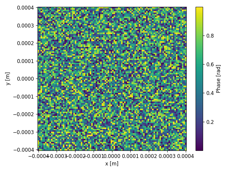
[95]:
#the initial arrays are two random matrices represented below
fig = plt.figure()
plt.pcolormesh(aperture_array_phase[0].XX, aperture_array_phase[0].YY, aperture_array_phase[0].aperture)
plt.colorbar(label ="Phase [rad]")
plt.xlabel("x [m]")
plt.ylabel("y [m]")
plt.tight_layout()
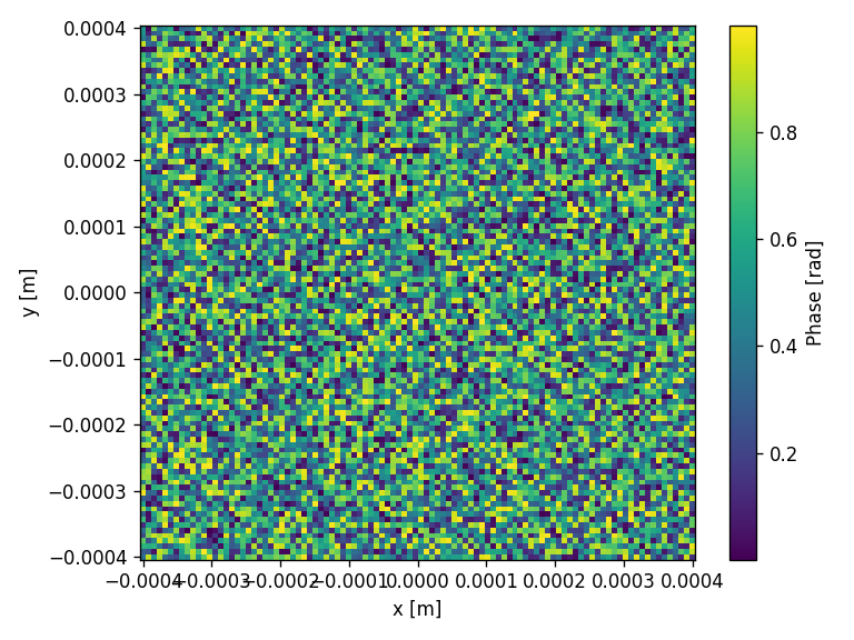
fig = plt.figure()
plt.pcolormesh(aperture_array_phase[1].XX, aperture_array_phase[1].YY, aperture_array_phase[1].aperture)
plt.colorbar(label ="Phase [rad]")
plt.xlabel("x [m]")
plt.ylabel("y [m]")
plt.tight_layout()
[96]:
prop_methods = ["bluestein", "bluestein"]
EXY_array2 = [moe.propagate.propagate_through_ensemble(ensemble, wavelength, propagation_methods_array=prop_methods) for wavelength in wavelength_array]
Surface #1
Progress: [####################] 100.0%
Elapsed: 0:00:00.008961
Surface #2
Progress: [####################] 100.0%
Elapsed: 0:00:00.009956
[97]:
x0_flatten = (np.array([aperture_array_phase[0].aperture.flatten(), aperture_array_phase[1].aperture.flatten()]) ).flatten()
x0_flatten.shape, a1_phase.shape
[97]:
((20000,), (100, 100))
[98]:
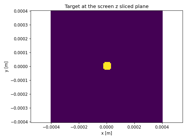
xi = np.arange(x_pixel)
yi = np.arange(y_pixel)
XX, YY = np.meshgrid(xi,yi, indexing='ij')

target = np.zeros((x_pixel, y_pixel))
target[np.where(((XX-x_pixel/2- 0)**2 + (YY-y_pixel/2-0)**2) < 4**2)] = 1

target_flat = target.flatten()

fig = plt.figure()
plt.pcolormesh(screen_array[-1].XX[:,:,-1], screen_array[-1].YY[:,:,-1], target )
plt.axis("equal")
plt.xlabel("x [m]")
plt.ylabel("y [m]")
plt.title("Target at the screen z sliced plane")
plt.tight_layout()
[99]:
def loss(x, mask, screen_array, wavelength, target, use_timer=False, propag="bluestein"):
    import jax.numpy as jnp

    #prop_x =  np.abs(moe.optimizer.propagate(np.reshape(x, (len(screen.x), len(screen.y))), mask, screen, wavelength, propagation_method=propag))
    xar1 = jnp.reshape(x[0:int(len(x)/2)], (len(screen_array[0].x), len(screen_array[0].y)))
    xar2 = jnp.reshape(x[int(len(x)/2):], (len(screen_array[0].x), len(screen_array[0].y)))
    xar=[xar1, xar2]

    prop_x = moe.optimizer.propagate(xar, aperture=aperture_array_phase, screen=screen_array , wavelength=wavelength_array, \
          mask_amp = aperture_array_amp, circ_radius=None, input_field="uniform", E0=1, \
          propagation_method=["ASM","ASM"], pad_factor=2, modedef = "czt", ensemble_mode=True , corr=1e5, use_timer=use_timer  )**2


    diff = jnp.abs(prop_x/jnp.sum(prop_x) - target/jnp.max(target))**2

    res = jnp.sum(diff)

    return res
[100]:
aperture = moe.generate.create_empty_aperture_from_aperture(asph2_mask_phase)
[101]:
solution = moe.optimizer.optimize(loss, x0_flatten, args1=[aperture, screen_array, wavelength, target, False], verbose = 1, ftol=1e-3,)

x = solution.x
`ftol` termination condition is satisfied.
Function evaluations 18, initial cost 1.0122e+03, final cost 4.1915e+02, first-order optimality 3.41e+00.
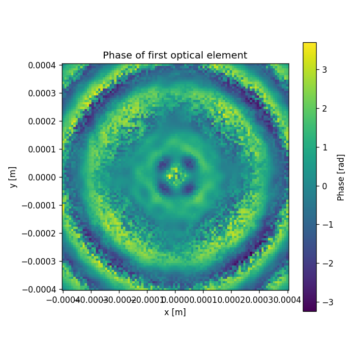
[102]:
d1 = np.reshape(x[0:int(len(x)/2)], (len(screen_array[0].x), len(screen_array[0].y)))
d2 = np.reshape(x[int(len(x)/2):], (len(screen_array[0].x), len(screen_array[0].y)))
fig = plt.figure(figsize = (6,6))
xar3 = np.reshape(d1, (x_pixel, y_pixel))
plt.pcolormesh(aperture_array_phase[0].XX, aperture_array_phase[0].YY, xar3)
plt.colorbar(label = "Phase [rad]", shrink=0.8)
plt.title("Phase of first optical element")
plt.xlabel("x [m]")
plt.ylabel("y [m]")
plt.gca().set_aspect('equal')
plt.tight_layout()
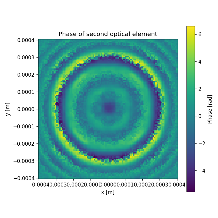
fig = plt.figure(figsize = (6,6))
xar4 = np.reshape(d2, (x_pixel, y_pixel))
plt.pcolormesh(aperture_array_phase[1].XX, aperture_array_phase[1].YY, xar4)
plt.colorbar(label = "Phase [rad]", shrink=0.8)
plt.title("Phase of second optical element")
plt.xlabel("x [m]")
plt.ylabel("y [m]")
plt.gca().set_aspect('equal')
plt.tight_layout()
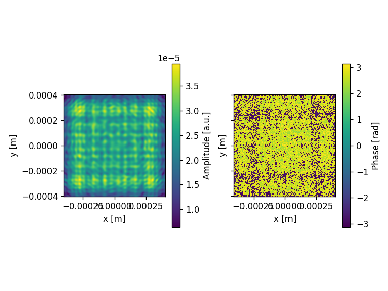
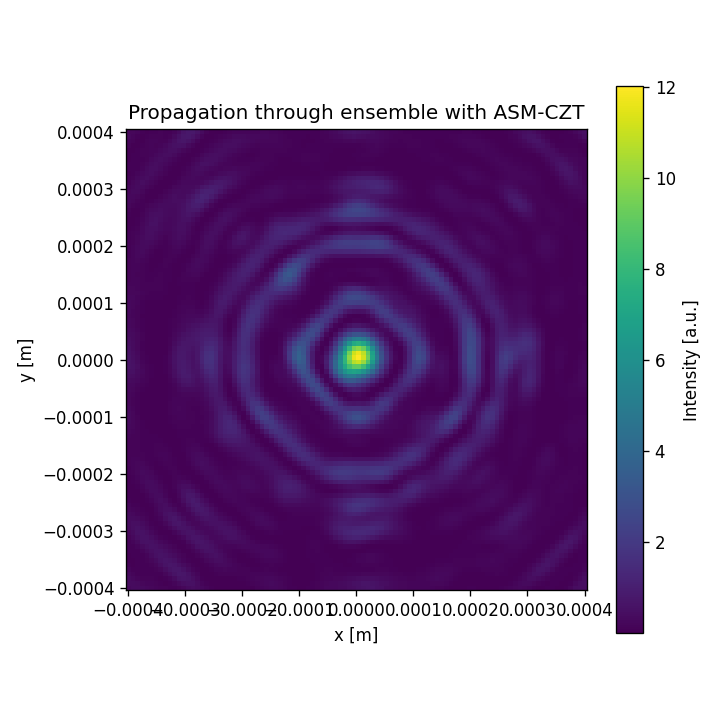
Ep = moe.optimizer.propagate(xar=[d1, d2], aperture=aperture_array_phase, screen=screen_array , wavelength=wavelength_array, \
mask_amp = aperture_array_amp, circ_radius=None, input_field="uniform", E0=1, \
propagation_method=["ASM","ASM"], pad_factor=2, modedef = "czt", ensemble_mode=True )
fig = plt.figure(figsize = (6,6))
plt.pcolormesh(screen_array[-1].XX[:,:,-1], screen_array[-1].YY[:,:,-1], (np.abs(Ep) )**2)
plt.colorbar(label = "Intensity [a.u.]", shrink=0.8)
plt.title("Propagation through ensemble with ASM-CZT")
plt.xlabel("x [m]")
plt.ylabel("y [m]")
plt.gca().set_aspect('equal')
plt.tight_layout()
Ep = moe.optimizer.propagate(xar=[d1, d2], aperture=aperture_array_phase, screen=screen_array , wavelength=wavelength_array, \
mask_amp = aperture_array_amp, circ_radius=None, input_field="uniform", E0=1, \
propagation_method=["bluestein","bluestein"], pad_factor=2, ensemble_mode=True , corr=1e10 )
fig = plt.figure(figsize = (6,6))
plt.pcolormesh(screen_array[-1].XX[:,:,-1], screen_array[-1].YY[:,:,-1], (np.abs(Ep) )**2)
plt.colorbar(label = "Intensity [a.u.]", shrink=0.8)
plt.title("Propagation through ensemble with Bluestein")
plt.xlabel("x [m]")
plt.ylabel("y [m]")
plt.gca().set_aspect('equal')
plt.tight_layout()
Ep = moe.optimizer.propagate(xar=[d1, d2], aperture=aperture_array_phase, screen=screen_array , wavelength=wavelength_array, \
mask_amp = aperture_array_amp, circ_radius=None, input_field="uniform", E0=1, \
propagation_method=["bluestein","ASM"], pad_factor=2, ensemble_mode=True , corr=1e10 )
fig = plt.figure(figsize = (6,6))
plt.pcolormesh(screen_array[-1].XX[:,:,-1], screen_array[-1].YY[:,:,-1], (np.abs(Ep) )**2)
plt.colorbar(label = "Intensity [a.u.]", shrink=0.8)
plt.title("Propagation through ensemble with Bluestein+ASM")
plt.xlabel("x [m]")
plt.ylabel("y [m]")
plt.gca().set_aspect('equal')
plt.tight_layout()
Elapsed: 0:00:00.065709
Elapsed: 0:00:00.075712
Elapsed: 0:00:00.043808
Elapsed: 0:00:00.033805
Elapsed: 0:00:00.051732
Elapsed: 0:00:00.062767


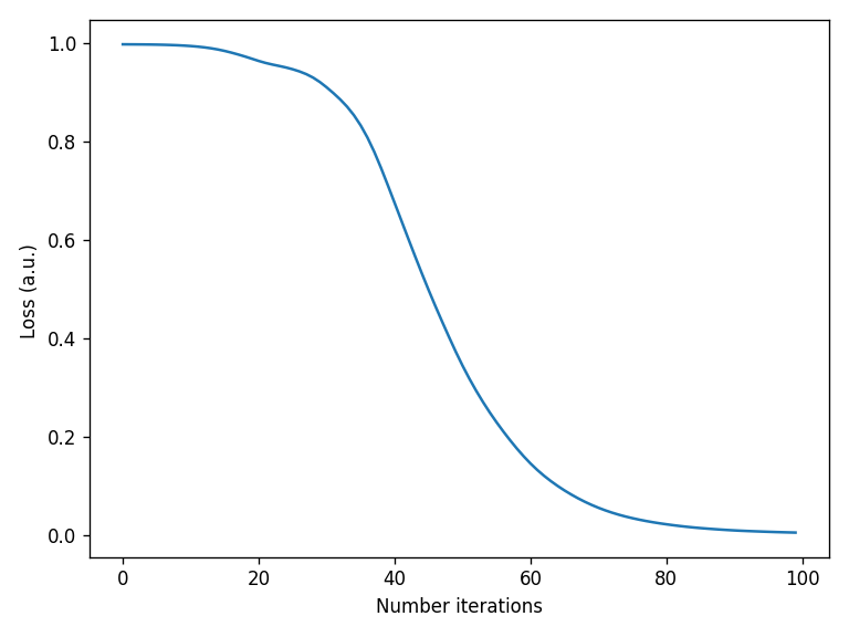
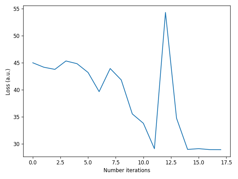
[103]:
loss_vector = solution.loss_history

plt.figure()
plt.plot(loss_vector)
plt.xlabel("Number iterations")
plt.ylabel("Loss (a.u.) ")
plt.tight_layout()
[ ]:
[ ]: