Metrics notebook

[1]:

# Notebook display options, change as your preference/system
%matplotlib inline
%config InlineBackend.print_figure_kwargs={'facecolor' : "w",'bbox_inches':None}

import matplotlib as mpl
mpl.rcParams['figure.dpi'] = 120

[2]:

# Notebook display options, change as your preference/syste

import sys
sys.path.insert(0,'..')
sys.path.insert(0,'../..')

from matplotlib import pyplot as plt
import numpy as np

from scipy.constants import micro, nano, milli

import pyMOE as moe
from pyMOE.generate import *
from pyMOE.propagate import *
from pyMOE.metrics import *
from pyMOE.optimizer import *
from pyMOE.ensemble import *

[3]:

# These metrics could be used to build specific loss functions

[4]:

#number of pixels
x_pixel = 100
y_pixel = 100


#size of the rectangular mask
aperture_width  = 50e-6 #m
aperture_height = 50e-6

pixsize = 1e-6 #m

wavelength = 500e-9 #m
focal_length = 150e-6

zmin = wavelength
zmax = 1.2* focal_length
nzs = 500

radius = aperture_width/2

# Create Aperture
aperture1 = moe.generate.create_empty_aperture(-aperture_width/2, aperture_width/2, x_pixel, -aperture_height/2, aperture_height/2, y_pixel)

# Populate Aperture with Fresnel mask
mask1 = moe.generate.fresnel_phase(aperture1, focal_length, wavelength )

#moe.plotting.plot_aperture(mask1)


##############
###Fresnel mask with a truncated circular aperture

# Create empty mask
aperture2 = moe.generate.create_empty_aperture(-aperture_width/2, aperture_width/2, x_pixel, -aperture_height/2, aperture_height/2, y_pixel)


# and truncate around radius
mask2 = moe.generate.fresnel_phase(aperture2, focal_length, wavelength, radius=radius)
#moe.plotting.plot_aperture(mask2)

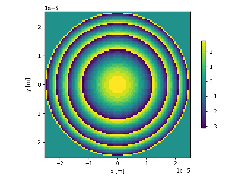
# Discretize mask in number of levels
# Select exact position of contours  in phase
phase_vals = np.linspace(-np.pi, np.pi, 16)

mask2.discretize(np.array( phase_vals)[:] )
#moe.plotting.plot_aperture(mask2)

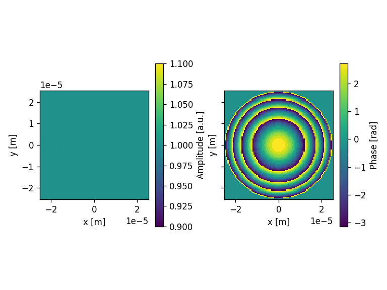
# Generate a uniform field
field = moe.field.create_empty_field_from_aperture(mask2)

field = moe.field.generate_uniform_field(field, E0=1)

# Modulates the field
field = moe.field.modulate_field(field, amplitude_mask=None, phase_mask=mask2 )

moe.plotting.plot_aperture(mask2)
moe.plotting.plot_field(field)

../_images/notebooks_Metrics_notebook_4_0.png

../_images/notebooks_Metrics_notebook_4_1.png

Point Spread Function (PSF)

[5]:

###Propagate field *10and calculate in plane YZ, using npix bins in Y
zmin = wavelength*10
zmax = 1.2* focal_length
nzs = 100

# Creates a screen in YZ plane with [-aperture_height/2, aperture_height/2] and [zmin, zmax] and
ymin, ymax = -aperture_height/2, aperture_height/2
xmin, xmax = -aperture_width/2, aperture_width/2


x_pixel, y_pixel = 100,100

x = np.linspace(xmin, xmax, x_pixel )
y = np.linspace(ymin, ymax, y_pixel )
z = np.linspace(zmin, zmax, nzs)


screen = moe.field.Screen(x,y,z)
sfreq = moe.metrics.spatial_freq_space(screen)
# Propagate the field
EXYZ = moe.propagate.Bluestein(field, screen, wavelength)

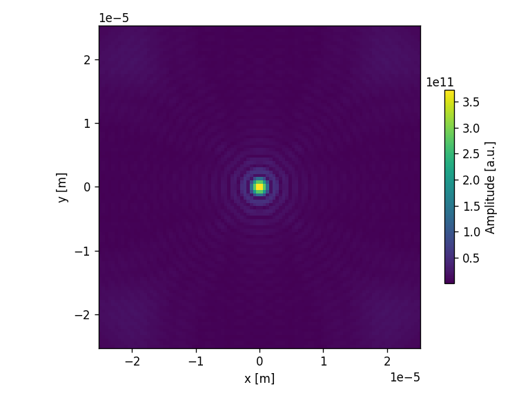
#This will show a PSF at the focal length
Exy = moe.field.Screen(x,y,z)
Exy.screen = np.reshape(EXYZ.screen[:,:, int(focal_length/zmax*nzs)], (x_pixel,y_pixel,1))

moe.plotting.plot_screen_XY(Exy, which='amplitude')

Progress: [####################] 100.0%
Elapsed: 0:00:00.452021

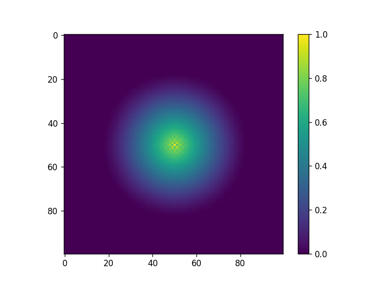
../_images/notebooks_Metrics_notebook_6_1.png

Optical Transfer Function (OTF)

[6]:

#Calculate the OTF out of focus and in focus
import scipy.fftpack as sfft

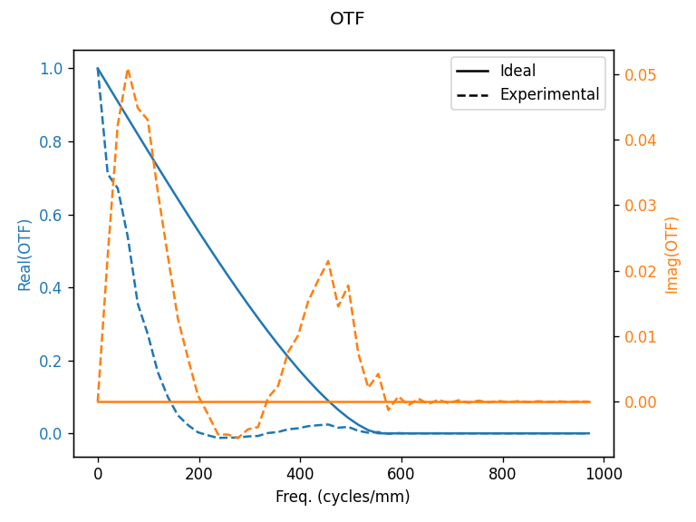
print("OTF from defocused PSF")
o1 = moe.metrics.calculate_OTF(np.abs(screen.screen[:,:,-1])**2 , plot_OTF=True)

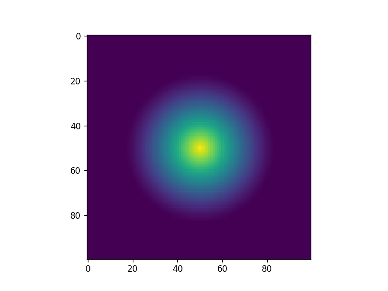
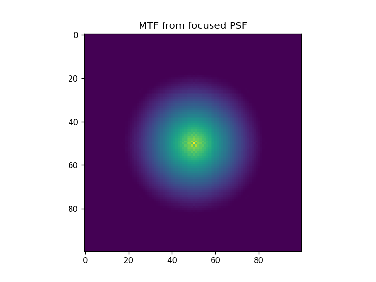
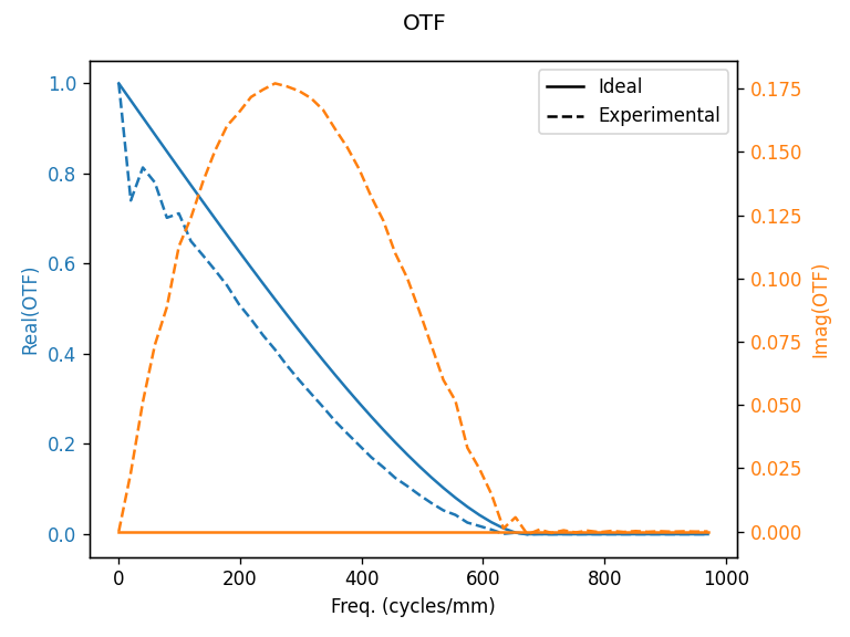
print("OTF from focused PSF")
o2 = moe.metrics.calculate_OTF(np.abs(Exy.screen[:,:,-1])**2  , plot_OTF=True)

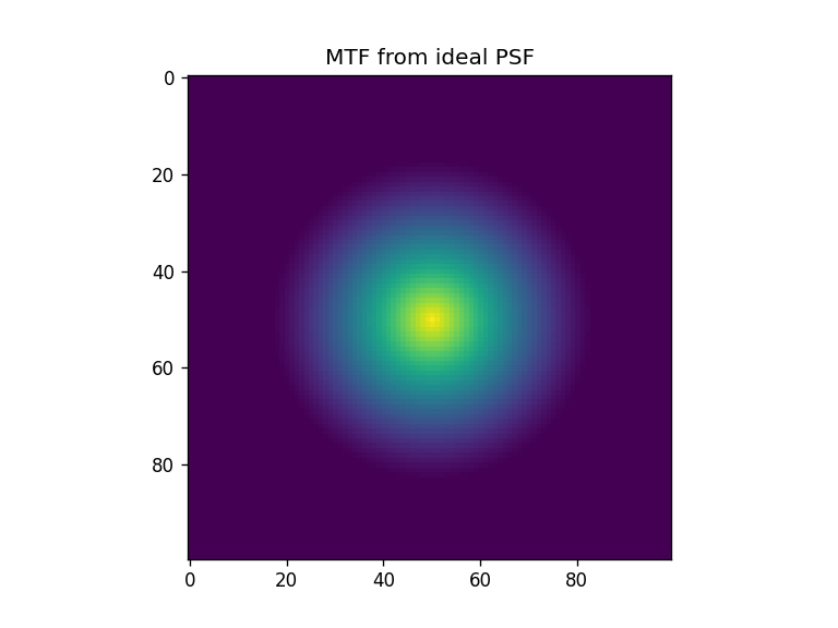
print("OTF for ideal (focused) PSF")

D = np.max(Exy.x)*2
OTF_ideal = moe.metrics.theoretical_ideal_OTF(Exy, D, wavelength, focal_length)


fig = plt.figure()
plt.imshow( OTF_ideal)

OTF from defocused PSF

../_images/notebooks_Metrics_notebook_8_1.png

OTF from focused PSF

../_images/notebooks_Metrics_notebook_8_3.png

OTF for ideal (focused) PSF

C:\Users\jcunha377\Desktop\pyMOE-main-v2.0\notebooks\8 - Metrics\../..\pyMOE\metrics.py:162: RuntimeWarning: invalid value encountered in arccos
  OTF = (2 / np.pi) * (np.arccos(rho / fc) - (rho / fc) * np.sqrt(1 - (rho / fc)**2))
C:\Users\jcunha377\Desktop\pyMOE-main-v2.0\notebooks\8 - Metrics\../..\pyMOE\metrics.py:162: RuntimeWarning: invalid value encountered in sqrt
  OTF = (2 / np.pi) * (np.arccos(rho / fc) - (rho / fc) * np.sqrt(1 - (rho / fc)**2))

[6]:

<matplotlib.image.AxesImage at 0x1921040b1d0>

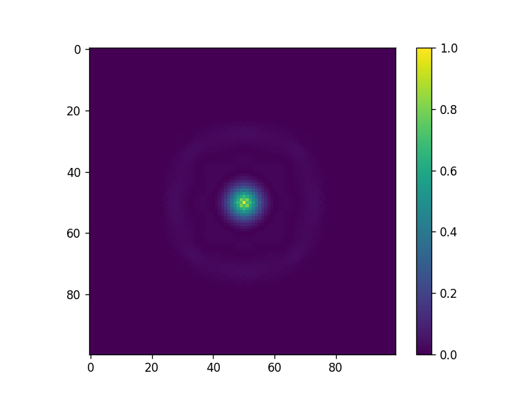
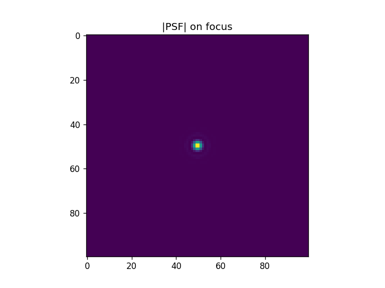
../_images/notebooks_Metrics_notebook_8_7.png

[7]:

plt.figure()

plt.title("|PSF| on focus")
plt.imshow(np.abs(Exy.screen)**2)

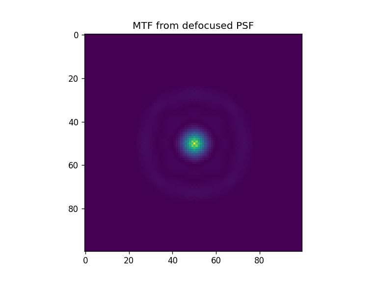
plt.figure()

plt.title("MTF from defocused PSF")
plt.imshow(np.abs(o1) )

plt.figure()
plt.title("MTF from focused PSF")
plt.imshow(np.abs(o2) )

plt.figure()
plt.title("MTF from ideal PSF")
plt.imshow(np.abs(OTF_ideal) )

[7]:

<matplotlib.image.AxesImage at 0x192104c82d0>

../_images/notebooks_Metrics_notebook_9_1.png

../_images/notebooks_Metrics_notebook_9_2.png

../_images/notebooks_Metrics_notebook_9_3.png

../_images/notebooks_Metrics_notebook_9_4.png

[8]:

max([max(Exy.x), max(Exy.y)]), Exy.z[0]

[8]:

(2.5e-05, 4.9999999999999996e-06)

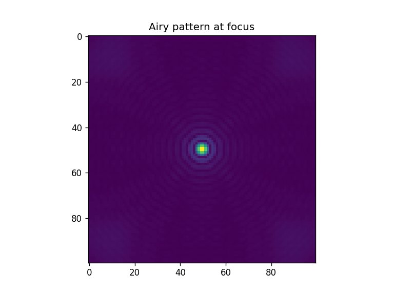
[9]:

fig= plt.figure()
plt.title("Airy pattern at focus")
plt.imshow(np.abs(Exy.screen) )

[9]:

<matplotlib.image.AxesImage at 0x1921072f810>

../_images/notebooks_Metrics_notebook_11_1.png

Modulation Transfer Function (MTF) and Phase Transfer Function (PTF) & Strehl ratio

[10]:

# MTF and OTF at DEFOCUSED PLANE

strehlv1 = moe.metrics.strehl_ratio(np.abs(screen.screen[:,:,-1] )**2, screen, max([max(Exy.x), max(Exy.y)])*2, wavelength, screen.z[-1], strehl_from_mtf=True, plot_MTF=True, plot_OTF=True)

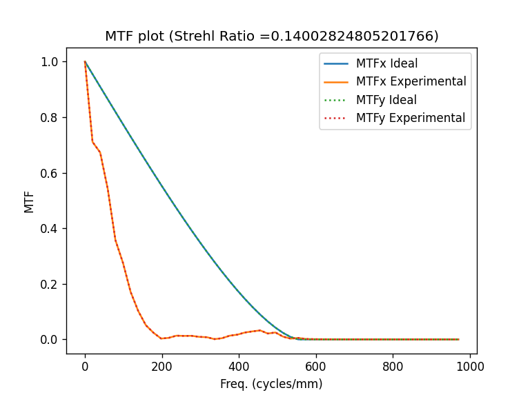
../_images/notebooks_Metrics_notebook_13_0.png

../_images/notebooks_Metrics_notebook_13_1.png

[11]:

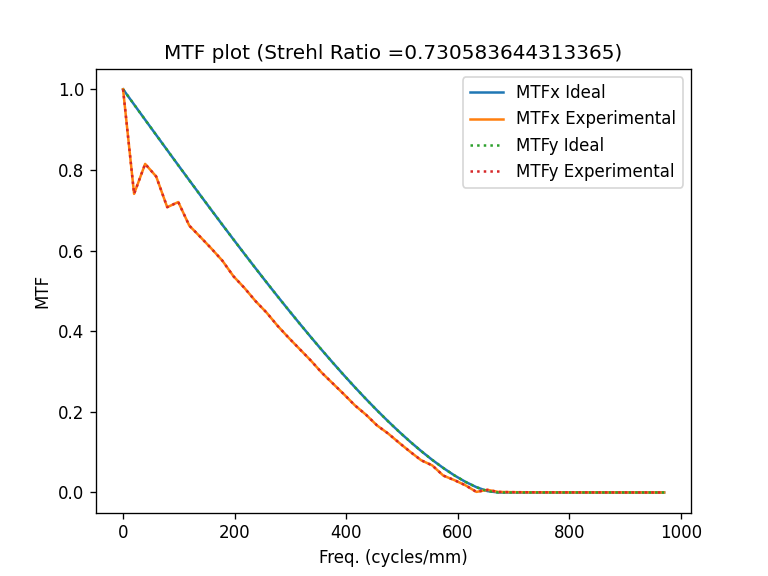
# MTF and OTF at FOCUSED PLANE

strehlv2 = moe.metrics.strehl_ratio(np.abs(Exy.screen[:,:,-1] )**2, Exy, max([max(Exy.x), max(Exy.y)])*2, wavelength, focal_length, strehl_from_mtf=True, plot_MTF=True, plot_OTF=True )

../_images/notebooks_Metrics_notebook_14_0.png

../_images/notebooks_Metrics_notebook_14_1.png

[12]:

# UNFOCUSED AND FOCUSED STREHL RATIOS
strehlv1, strehlv2

[12]:

(0.14002824805201766, 0.84009513106553)

[13]:

#moe.metrics.strehl_ratio(np.abs(Exy.screen[:,:,-1])**2, screen, max([max(screen.x), max(screen.y)])*2, wavelength, focal_length, plot_MTF=True) ,\
#moe.metrics.strehl_ratio(np.abs(Exy.screen[:,:,-1])**2, Exy, max([max(Exy.x), max(Exy.y)])*2, wavelength, focal_length, plot_MTF=True)

Encircled energy

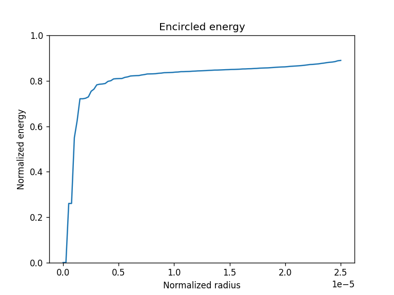
[14]:

center=(0,0)

parray = np.linspace(0, aperture_width/2, 100)

enarray = [moe.metrics.encircled_energy(Exy, p) for p in parray]
enmax = moe.metrics.encircled_energy(Exy, 1.01)

fig = plt.figure()

plt.plot(parray, enarray/enmax)
plt.ylim([0,1])
plt.xlabel("Normalized radius")
plt.ylabel("Normalized energy")
plt.title("Encircled energy")
#plt.yscale("log")

#This is not exactly one, because other energy is lost to the square parts of the sensor


#The energy plateus at 0.5e-6, so makes sense to use that as p

[14]:

Text(0.5, 1.0, 'Encircled energy')

../_images/notebooks_Metrics_notebook_18_1.png

[15]:

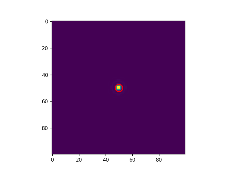
XY=np.abs(Exy.screen[:,:,-1])**2

largestpeak_height , largestpeak_width, position = moe.metrics.find_FWHM_2d(XY, prominence=0.5)

largestpeak_height , largestpeak_width, position

[15]:

(1.3879175930586803e+22, 5.499479222542831, array([50, 50], dtype=int64))

[16]:

from matplotlib.patches import Circle

fig = plt.figure()

plt.imshow(np.abs(XY))

# Get image dimensions
height, width = XY.shape

# Add central circle
circle = Circle((position[0], position[1]), radius=largestpeak_width/2, color='red', fill=False, linewidth=2)
plt.gca().add_patch(circle)

[16]:

<matplotlib.patches.Circle at 0x19210f42390>

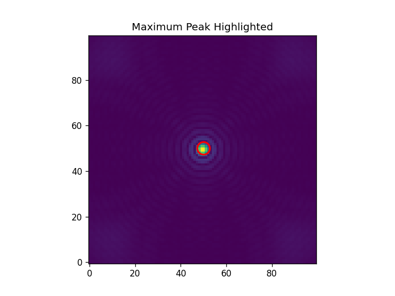
../_images/notebooks_Metrics_notebook_20_1.png

[17]:

largestpeak_height , largestpeak_width, largestpeak_position = moe.metrics.find_FWHM_2d(np.abs(Exy.screen[:,:,-1])**2, prominence=0.5)


from matplotlib.patches import Circle

fig, ax = plt.subplots()
ax.imshow(np.abs(Exy.screen[:,:,-1]),  origin='lower')

# Draw the circle
circle = Circle((largestpeak_position[0], largestpeak_position[1]),  # x, y
                radius=largestpeak_width/2, color='red', fill=False, linewidth=2)
ax.add_patch(circle)

# Optional: mark the center
#ax.plot(largestpeak_position[0], largestpeak_position[1], 'ro')  # center dot

plt.title("Maximum Peak Highlighted")
plt.show()

../_images/notebooks_Metrics_notebook_21_0.png

[18]:

##encircled energy at 1 FWHM

one_fwhm = moe.metrics.encircled_energy(Exy, (width/2)*pixsize)/moe.metrics.encircled_energy(Exy, 1.01)

##encircled energy at 0.5 FWHM

half_fwhm = moe.metrics.encircled_energy(Exy, (width/2)*pixsize*0.5)/moe.metrics.encircled_energy(Exy, 1.01)

(width/2)*pixsize, one_fwhm, half_fwhm
#This is consistent with the plateauing that is seen in the encircled energy

[18]:

(4.9999999999999996e-05, 1.0, 0.8898340172814078)

Ensquared energy

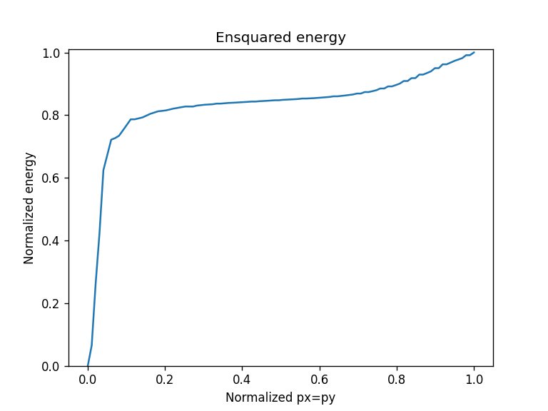
[19]:

center=(0,0)

parray = np.linspace(0, aperture_width/2, 100)

enarray = [moe.metrics.ensquared_energy(Exy, p, p) for p in parray]
enmax = moe.metrics.ensquared_energy(Exy, 1,1)

fig = plt.figure()

plt.plot(parray/(aperture_width/2), enarray/enmax)
plt.ylim([0,1.01])
plt.xlabel("Normalized px=py")
plt.ylabel("Normalized energy")
plt.title("Ensquared energy")

[19]:

Text(0.5, 1.0, 'Ensquared energy')

../_images/notebooks_Metrics_notebook_24_1.png

Focusing Efficiency

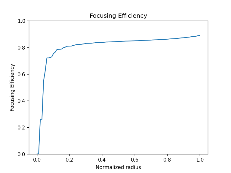
[20]:

center=(0,0)

parray = np.linspace(0, aperture_width/2, 100)

#Should give the same as the enclircled energy
farray1 = [moe.metrics.focus_efficiency(Exy, p,  encircled_energy(Exy, 1.01),center=(0,0),) for p in parray]

fig = plt.figure()

plt.plot(parray/(aperture_width/2), farray1)
plt.ylim([0,1])
plt.xlabel("Normalized radius")
plt.ylabel("Focusing Efficiency")
plt.title("Focusing Efficiency")
#plt.yscale("log")

[20]:

Text(0.5, 1.0, 'Focusing Efficiency')

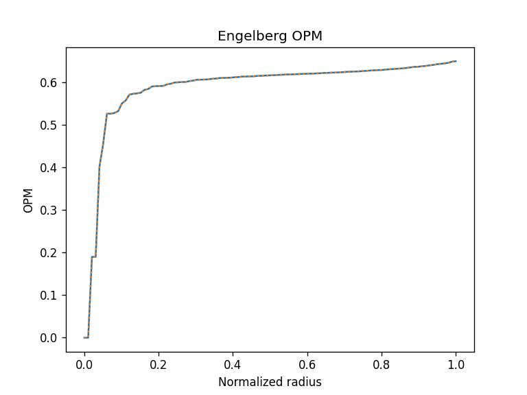
../_images/notebooks_Metrics_notebook_26_1.png

Optical Performance Metric (OPM)

[21]:

#Engelberg metric, check original paper for more detail

center=(0,0)

parray = np.linspace(0, aperture_width/2, 100)

farray2 = [moe.metrics.Engelberg_OPM(Exy, p,  moe.metrics.encircled_energy(Exy, 1.01),1, wavelength, z = focal_length) for p in parray]
strehlr = moe.metrics.strehl_ratio(np.abs(Exy.screen[:,:,-1])**2, Exy, max([max(Exy.x), max(Exy.y)])*2, wavelength, focal_length, plot_MTF=True)

fig = plt.figure()

plt.plot(parray/(aperture_width/2), farray2)
plt.plot(parray/(aperture_width/2), strehlr*np.array(farray1), ':' )
#plt.ylim([0,1])
plt.xlabel("Normalized radius")
plt.ylabel("OPM")
plt.title("Engelberg OPM")

[21]:

Text(0.5, 1.0, 'Engelberg OPM')

../_images/notebooks_Metrics_notebook_28_1.png

../_images/notebooks_Metrics_notebook_28_2.png

[22]:

#strehlr = moe.metrics.strehl_ratio(np.abs(Exy.screen[:,:,0])**2, screen, max([max(Exy.x), max(Exy.y)])*2, wavelength, focal_length, plot_MTF=True)

Comparisons to theoretical (analytical)

[23]:

# Make circular apertures (returns also the 2D array)

wavelength = 1550e-9 #m


pixsize = 1e-6
x_pixel = 64
y_pixel = 64

aperture_width  = x_pixel*pixsize
aperture_height = y_pixel*pixsize

radius = 0.5*x_pixel*pixsize #m
zdist = 10*radius #m

#screen size
xminus = -400e-3 #m
xplus = 400e-3 #m


# Define Aperture
aperture = moe.generate.create_empty_aperture(-aperture_width/2, aperture_width/2, x_pixel, -aperture_height/2, aperture_height/2, y_pixel)

# Populate Aperture from phase mask
mask = moe.generate.circular_aperture(aperture, radius=radius, center=(0,0))

# Define Phase mask
mask_phase = moe.generate.create_empty_aperture_from_aperture(aperture)
mask_phase.aperture = mask.aperture*np.pi


# Plot the circular mask
#moe.plotting.plot_aperture(mask_phase)

[24]:

###Propagate field *10and calculate in plane YZ, using npix bins in Y
zdist=100*radius
zmin = wavelength*10
zmax = 1.2* zdist
nzs = 500

focal_length = 3.5e-4


# Creates a screen in YZ plane with [-aperture_height/2, aperture_height/2] and [zmin, zmax] and
ymin, ymax = -aperture_height/2, aperture_height/2
xmin, xmax = -aperture_width/2, aperture_width/2

x = np.linspace(xmin, xmax, x_pixel)
y = np.linspace(ymin, ymax, y_pixel)
z = np.linspace(zmin, zmax, nzs)

# Calculates a field to use with the calculated mask

# Initialize a Field from the Aperture mask
field = moe.field.create_empty_field_from_aperture(mask)

# Generate a uniform field
field = moe.field.generate_uniform_field(field, E0=1e5)

# Or Gaussian field is also available
#field = moe.field.generate_gaussian_field(field, E0=1, w0=100*micro)

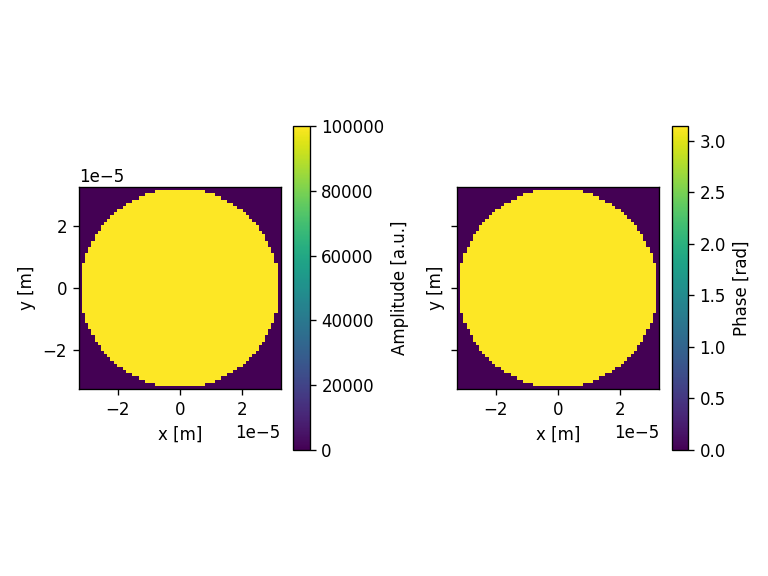
# Modulates the field with a given aperture that can be used either as an amplitude mask or a phase mask
field = moe.field.modulate_field(field, amplitude_mask=mask, phase_mask=mask_phase)

###Propagate field *10and calculate in plane YZ, using npix bins in Y
zdist=100*radius
zmin = wavelength*10
zmax = 1.2* zdist
nzs = 500

focal_length = 4.5e-4


# Creates a screen in YZ plane with [-aperture_height/2, aperture_height/2] and [zmin, zmax] and
ymin, ymax = -aperture_height/2, aperture_height/2
xmin, xmax = -aperture_width/2, aperture_width/2

x = np.linspace(xmin, xmax, x_pixel)
y = np.linspace(ymin, ymax, y_pixel)
z = np.linspace(zmin, zmax, nzs)

# Calculates a field to use with the calculated mask

# Initialize a Field from the Aperture mask
field = moe.field.create_empty_field_from_aperture(mask)

# Generate a uniform field
field = moe.field.generate_uniform_field(field, E0=1e5)

# Or Gaussian field is also available
#field = moe.field.generate_gaussian_field(field, E0=1, w0=100*micro)

# Modulates the field with a given aperture that can be used either as an amplitude mask or a phase mask
field = moe.field.modulate_field(field, amplitude_mask=mask, phase_mask=mask_phase)

# Plots the field (amplitude and phase)
moe.plotting.plot_field(field)

plt.tight_layout()
plt.show()


screen = moe.field.Screen(x,y,z)

# Propagate the field
EXYZ = moe.propagate.Bluestein(field, screen, wavelength)

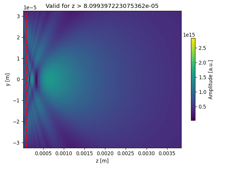
Eyz = moe.field.Screen(0,y,z)
Eyz.screen = np.reshape(EXYZ.screen[:,int(y_pixel/2), :], np.shape(Eyz.screen[:, :, :]))

moe.plotting.plot_screen_YZ(Eyz, which='amplitude')

limitx = moe.propagate.Fresnel_criterion(wavelength,radius)
plt.vlines(limitx, -radius, radius, colors='red', linestyles='dashed', lw=2)

plt.title("Valid for z > "+str(limitx))

plt.show()

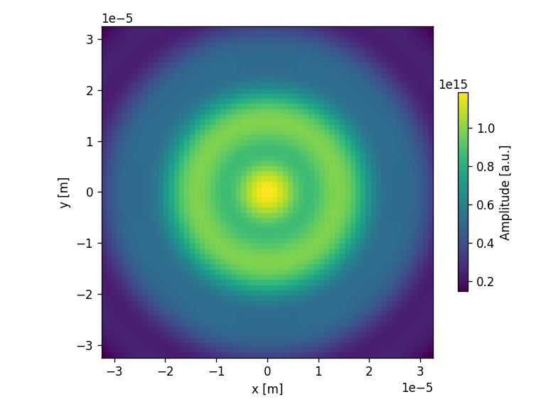
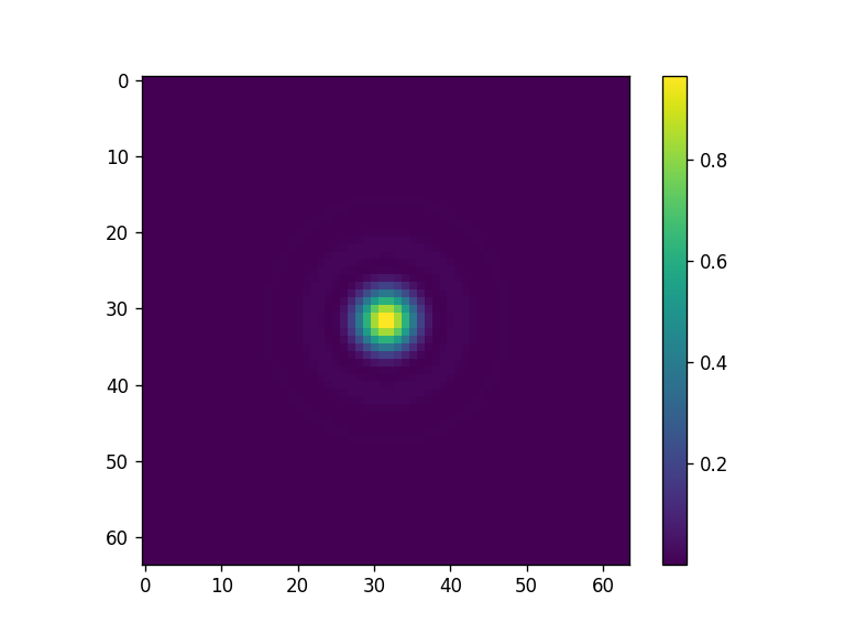
Exy = moe.field.Screen(x,y,[focal_length])
Exy.screen = np.reshape(EXYZ.screen[:,:, int(focal_length/zmax*nzs)], np.shape(Exy.screen[:, :, :]))

moe.plotting.plot_screen_XY(Exy, which='amplitude')

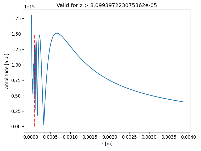
Ezz = moe.field.Screen(0,0,z)
Ezz.screen = np.reshape(EXYZ.screen[int(x_pixel/2),int(y_pixel/2),:], np.shape(Ezz.screen[:, :, :]))

moe.plotting.plot_screen_ZZ(Ezz, which='amplitude')

limitx = moe.propagate.Fresnel_criterion(wavelength,radius)
plt.vlines(limitx, 0, np.max(Ezz.screen), colors='red', linestyles='dashed', lw=2)

plt.title("Valid for z > "+str(limitx))

plt.show()

../_images/notebooks_Metrics_notebook_32_0.png

Progress: [####################] 100.0%
Elapsed: 0:00:01.039527

../_images/notebooks_Metrics_notebook_32_2.png

C:\ProgramData\anaconda3\Lib\site-packages\numpy\ma\core.py:3375: ComplexWarning: Casting complex values to real discards the imaginary part
  _data[indx] = dval

../_images/notebooks_Metrics_notebook_32_4.png

../_images/notebooks_Metrics_notebook_32_5.png

[25]:

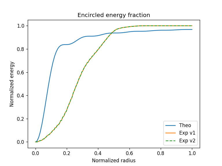
## RESULT TO BE CHECKED, MISMATCH MAYBE DUE TO DISTINCT DEFINITION OF RADIUS p ??

center=(0,0)

parray1 = np.linspace(0, aperture_width, 200)

enarray = [moe.metrics.encircled_energy(Exy, p) for p in parray1]
enmax = moe.metrics.encircled_energy(Exy, 1.01)

parray2 = np.linspace(0, aperture_width*10, 100)
enarray_theo = [moe.metrics.theoretical_encircled_energy(Exy, p) for p in parray2]
enmaxtheo = moe.metrics.theoretical_encircled_energy(Exy, 1.01)

enarray2 = [moe.metrics.encircled_energy(Exy, p) for p in parray1]
enmax2 = moe.metrics.encircled_energy(Exy, 1.01)

fig = plt.figure()

plt.plot(parray2/parray2.max(), enarray_theo/enmaxtheo, label="Theo")
plt.plot(parray1/parray1.max(), enarray/enmax, label = "Exp v1")

plt.plot(parray1/parray1.max(), enarray2/enmax2 , '--', label ="Exp v2")

plt.xlabel("Normalized radius")
plt.ylabel("Normalized energy")
plt.title("Encircled energy fraction")

plt.legend()

#This is not exactly one, because other energy is lost to the square parts of the sensor

[25]:

<matplotlib.legend.Legend at 0x1920b3723d0>

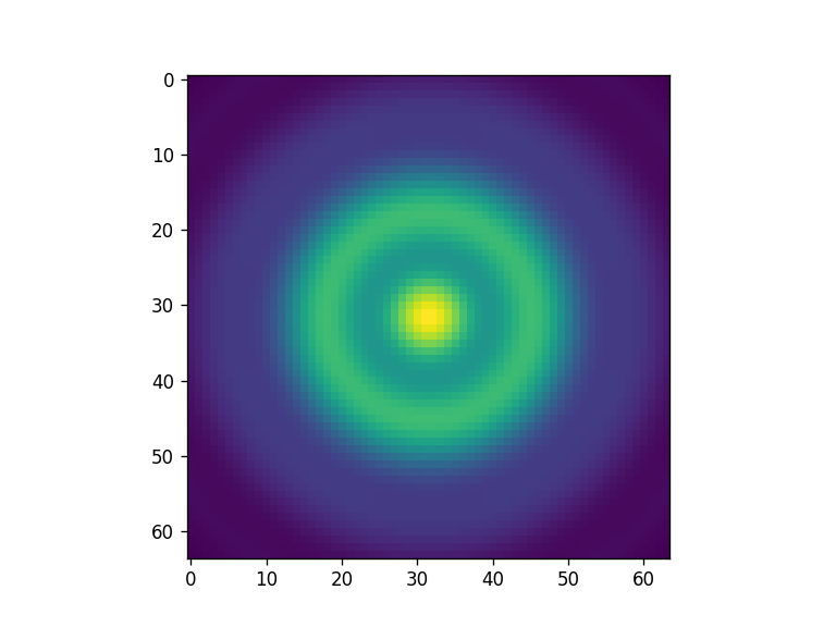
../_images/notebooks_Metrics_notebook_33_1.png

[26]:

fig = plt.figure()
plt.imshow(np.abs(Exy.screen[:,:,-1])**2)

[26]:

<matplotlib.image.AxesImage at 0x19210c28750>

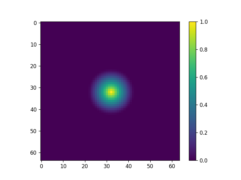
../_images/notebooks_Metrics_notebook_34_1.png

[27]:

#Sanity check with theoretical Airy pattern MTF,
# here the theoretical and calculated MTFs should give the same with unitary Strehl ratio

D = np.max(Exy.x)*2

wavelength = 200e-9  # Wavelength in meters (e.g., 550 nm)

intensity_circular = intensity_theo_Airy(screen, D*2, wavelength, z=1)


fig = plt.figure()
plt.imshow(intensity_circular  )
plt.colorbar()

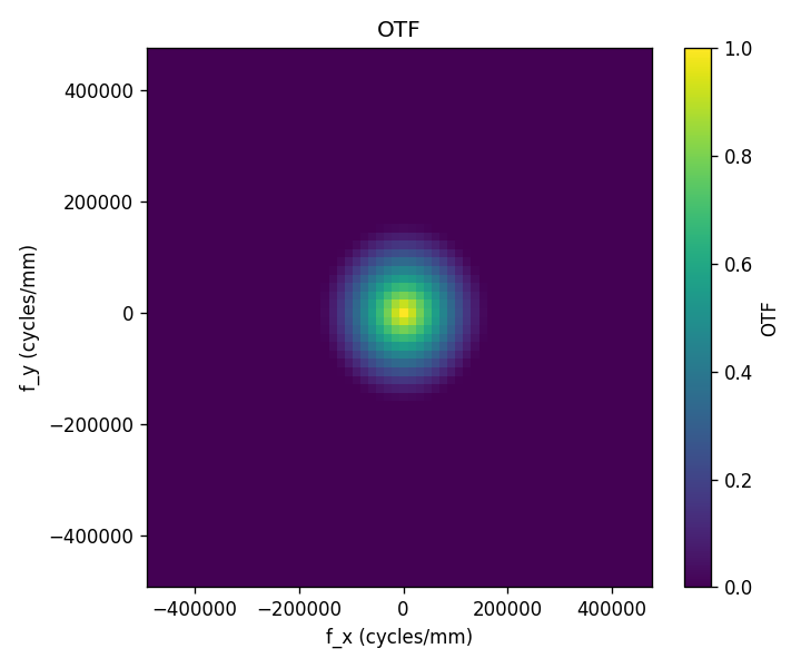
OTF_circular = calculate_OTF(intensity_circular)


fig = plt.figure()
plt.imshow(np.abs(OTF_circular) )
plt.colorbar()

fig = plt.figure()

N = 512
dx = 10e-6  # pixel pitch in meters
dy = 10e-6


# Plot
plt.figure(figsize=(6, 5))
plt.imshow(np.abs(OTF_circular), extent=(np.min(Exy.fx), np.max(Exy.fx), np.min(Exy.fy), np.max(Exy.fy)),
           origin='lower', cmap='viridis', aspect='auto')
plt.colorbar(label='OTF')
plt.xlabel('f_x (cycles/mm)')
plt.ylabel('f_y (cycles/mm)')
plt.title('OTF')
plt.tight_layout()
plt.show()

../_images/notebooks_Metrics_notebook_35_0.png

../_images/notebooks_Metrics_notebook_35_1.png

<Figure size 768x576 with 0 Axes>

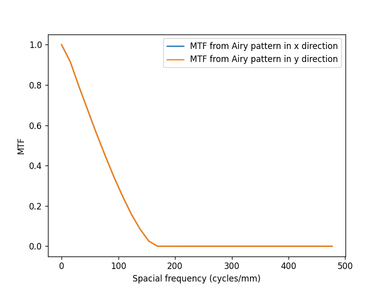
../_images/notebooks_Metrics_notebook_35_3.png

[28]:

mtf, mtfx1, mtfy1 = moe.metrics.MTF_from_OTF(OTF_circular)


fx, fy = screen.fx*1e-3, screen.fy *1e-3

fig = plt.figure()
plt.plot(fx[np.where(fx>=0)],  mtfx1, label="MTF from Airy pattern in x direction")
plt.plot(fy[np.where(fy>=0)],  mtfy1, label="MTF from Airy pattern in y direction")
plt.xlabel("Spacial frequency (cycles/mm)")
plt.ylabel("MTF")

plt.legend()

[28]:

<matplotlib.legend.Legend at 0x1920bfa16d0>

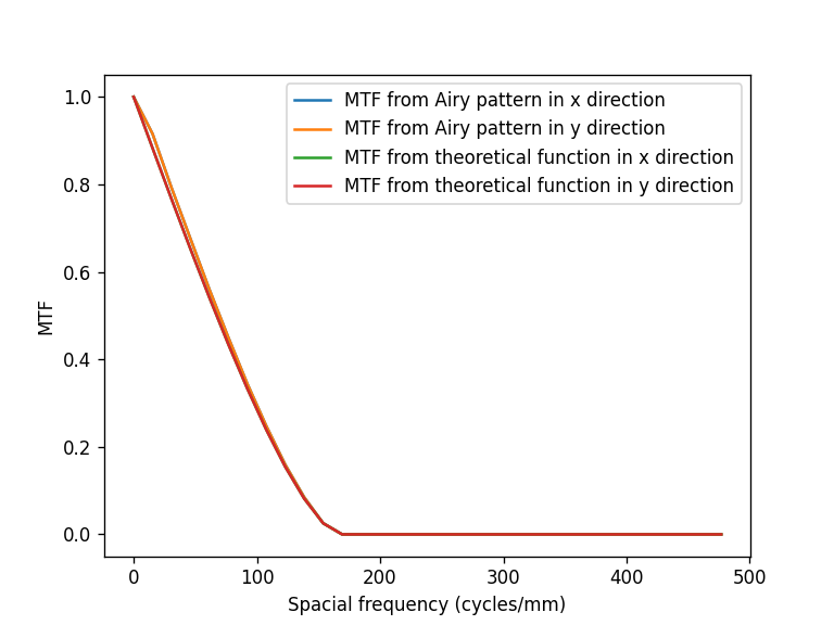
../_images/notebooks_Metrics_notebook_36_1.png

[29]:

otf = moe.metrics.theoretical_ideal_OTF(screen, D*2, wavelength, screen.z[-1])

mtf, mtfx2, mtfy2 = moe.metrics.MTF_from_OTF(otf)

[30]:

fx = screen.fx*1e-3
fy = screen.fy*1e-3

fig = plt.figure()
plt.plot(fx[np.where(fx>=0)],  mtfx1, label="MTF from Airy pattern in x direction")
plt.plot(fy[np.where(fy>=0)],  mtfy1, label="MTF from Airy pattern in y direction")
plt.plot(fx[np.where(fx>=0)],  mtfx2, label="MTF from theoretical function in x direction")
plt.plot(fy[np.where(fy>=0)],  mtfy2, label="MTF from theoretical function in y direction")
plt.xlabel("Spacial frequency (cycles/mm)")
plt.ylabel("MTF")

plt.legend()

[30]:

<matplotlib.legend.Legend at 0x1920ba0ab10>

../_images/notebooks_Metrics_notebook_38_1.png

[31]:

#This should give 1

moe.metrics.strehl_ratio(intensity_circular, screen, D*2, wavelength, z = screen.z[-1])

[31]:

0.998781221220814

[ ]: