Example notebook for optimize module
In the following we exemplify how to utilize the optimize module of pyMOE which uses gradient descent methods for inverse design of masks.
The idea is that the mask pixels can be iteratively changed to minimize of a loss function which evaluates the simulated propagated field from the mask against a target response. A gradient descent method changes the mask pixels iteratively in the direction of the gradient until a certain tolerance is met. Some metrics can be used for loss function constructions. Examples of simple loss functions are the root mean square error (RMSE) or the maximum likelihood estimator. pyMOE optimize module calculates the gradient through JAX package, employing scipy or optax (JAX) optimization frameworks, being extremelly versatile, allowing the user to pick different propagation methods for the task.
[76]:
# Notebook display options, change as your preference/system
%matplotlib inline
%config InlineBackend.print_figure_kwargs={'facecolor' : "w",'bbox_inches':None}

import matplotlib as mpl
mpl.rcParams['figure.dpi'] = 120
[77]:
import sys
sys.path.insert(0,'..')
sys.path.insert(0,'../..')

from matplotlib import pyplot as plt
import numpy as np

from scipy.constants import micro, nano, milli

import pyMOE as moe
[78]:
# auto reload
%load_ext autoreload
%autoreload 2
The autoreload extension is already loaded. To reload it, use:
  %reload_ext autoreload
[132]:
#number of pixels
x_pixel = 100
y_pixel = 100

#size of the mask
aperture_width  = 50e-6 #m
aperture_height = 50e-6

pixsize = 1e-6 #m

wavelength = 500e-9 #m
Initializations
[133]:
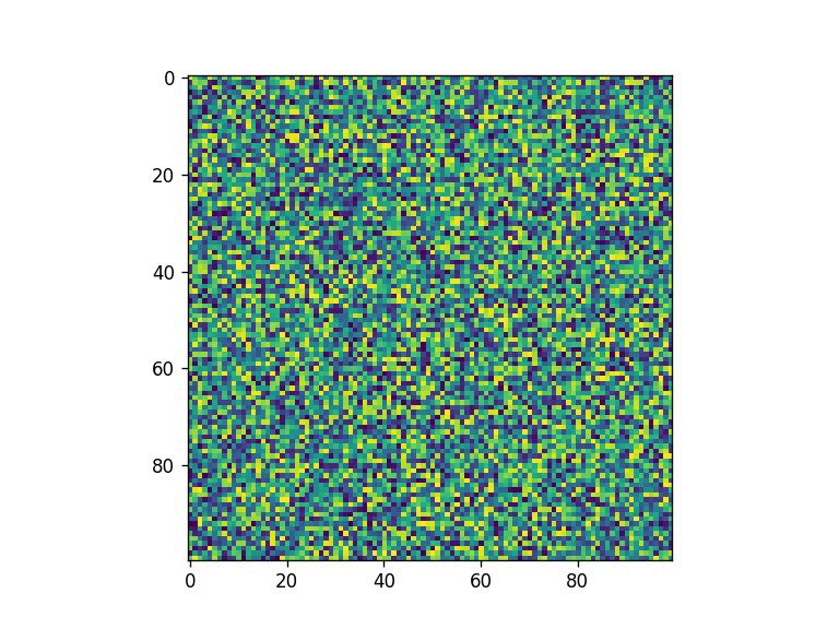
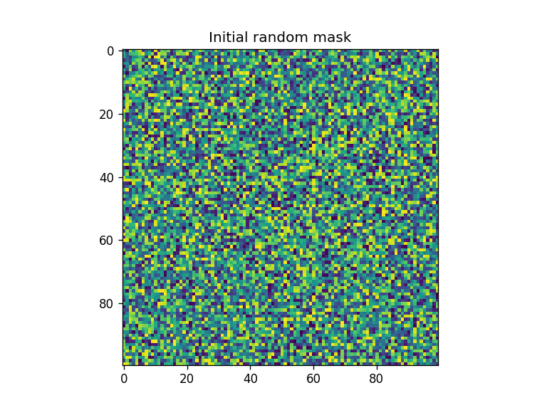
#Create initial random pixel distribution
x0 = np.random.rand(x_pixel, y_pixel)
x0_flatten = x0.flatten()

fig = plt.figure()
plt.imshow(x0)
[133]:
<matplotlib.image.AxesImage at 0x183a5d40f50>
[134]:
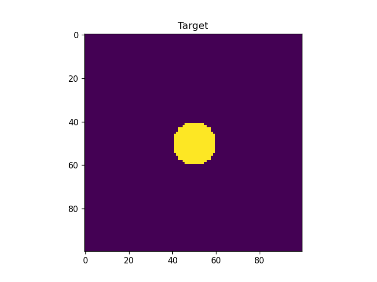
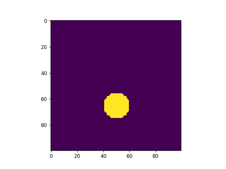
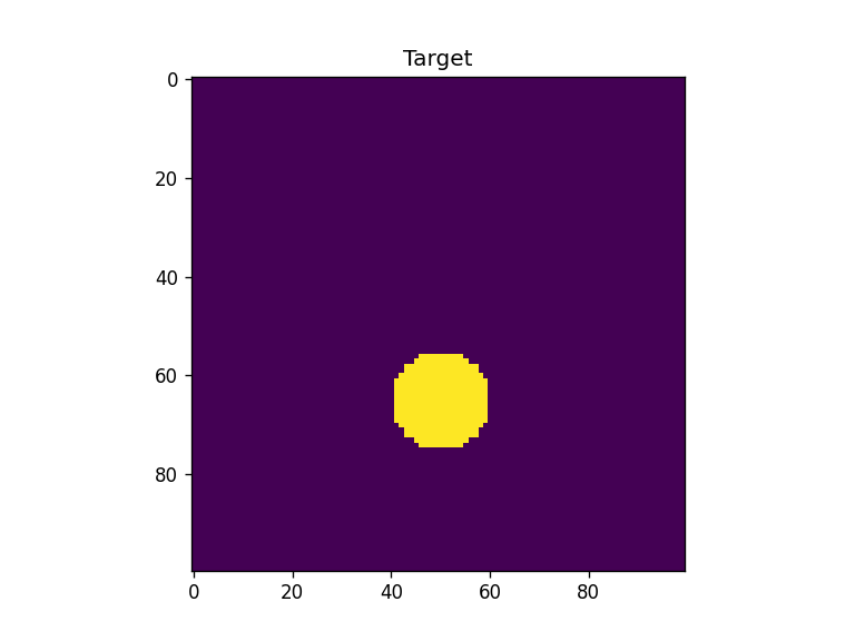
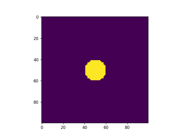
#create target matrix (central cricular pattern)
xi = np.arange(x_pixel)
yi = np.arange(y_pixel)
XX, YY = np.meshgrid(xi,yi)

target = np.zeros((x_pixel, y_pixel))
target[np.where(((XX-x_pixel/2)**2 + (YY-y_pixel/2)**2) < 10**2)] = 1

target_flat = target.flatten()

fig = plt.figure()
plt.imshow(target)
[134]:
<matplotlib.image.AxesImage at 0x183a5fd8d90>

Optimization framework
The optimization framework passes through the definition of loss functions. Here simply they compare the propagation against a defined target. The loss function takes the propagation method as parameter, so it that different parameters can be tested.
[82]:
#Define loss functions
def mseloss(x, mask, screen, wavelength, target, propag="bluestein"):
    import jax.numpy as jnp

    prop_x =  jnp.abs(moe.optimizer.propagate(jnp.reshape(x, (len(screen.x), len(screen.y))), mask, screen, wavelength, propagation_method=propag))

    diff = jnp.abs(prop_x/jnp.sum(prop_x) - target/jnp.max(target))**2

    res = jnp.mean(diff)

    return res


def logloss(x, mask, screen, wavelength, target=target_flat, propag="bluestein", use_timer=True):
    import jax.numpy as jnp

    prop_x = jnp.abs(moe.optimizer.propagate(jnp.reshape(x, (x_pixel, y_pixel)), mask, screen, wavelength, propagation_method=propag, use_timer=use_timer).flatten())
    prop_x = jnp.reshape(prop_x, (x_pixel, y_pixel))
    midx, midy = int(x_pixel/2), int(y_pixel/2)
    target = jnp.reshape(target, (x_pixel, y_pixel))

    res = jnp.log(np.sum(((prop_x/jnp.max(prop_x)/(prop_x[(midx,midy)]/jnp.max(prop_x)) - target/jnp.max(target))**2)))

    return res
[83]:
# Create Aperture
aperture = moe.generate.create_empty_aperture(-aperture_width/2, aperture_width/2, x_pixel, -aperture_height/2, aperture_height/2, y_pixel)
[84]:
# Creates a screen in YZ plane with [-aperture_height/2, aperture_height/2] at zdist
ymin, ymax = -aperture_height/2, aperture_height/2
xmin, xmax = -aperture_width/2, aperture_width/2

zdist = 0.00015

x = np.linspace(xmin, xmax, x_pixel)
y = np.linspace(ymin, ymax, y_pixel)
z = np.array([zdist])

screen = moe.Screen(x,y,z)
[85]:
#optimize using the optimizer module  and Bluestein propagation (default)
# the initial guess is the randomly initialized x0
solution = moe.optimizer.optimize(mseloss, x0_flatten, args1=[aperture, screen, wavelength, target], verbose = 1, ftol=1e-4, )
Elapsed: 0:00:00.015930
Elapsed: 0:00:00.014436
Elapsed: 0:00:00.040322
Elapsed: 0:00:00.015432
Elapsed: 0:00:00.015930
Elapsed: 0:00:00.040323
Elapsed: 0:00:00.014437
Elapsed: 0:00:00.014436
Elapsed: 0:00:00.040326
Elapsed: 0:00:00.014935
Elapsed: 0:00:00.017424
Elapsed: 0:00:00.045301
Elapsed: 0:00:00.014935
Elapsed: 0:00:00.015432
Elapsed: 0:00:00.039852
Elapsed: 0:00:00.014436
Elapsed: 0:00:00.014934
Elapsed: 0:00:00.039327
Elapsed: 0:00:00.016428
Elapsed: 0:00:00.014438
Elapsed: 0:00:00.046794
Elapsed: 0:00:00.019913
Elapsed: 0:00:00.016926
Elapsed: 0:00:00.039328
Elapsed: 0:00:00.014935
Elapsed: 0:00:00.014436
Elapsed: 0:00:00.038830
Elapsed: 0:00:00.014934
Elapsed: 0:00:00.016926
Elapsed: 0:00:00.041318
Elapsed: 0:00:00.014935
Elapsed: 0:00:00.014436
Elapsed: 0:00:00.040821
Elapsed: 0:00:00.015930
Elapsed: 0:00:00.029371
Elapsed: 0:00:00.041319
Elapsed: 0:00:00.014436
Elapsed: 0:00:00.013939
Elapsed: 0:00:00.050279
Elapsed: 0:00:00.015432
Elapsed: 0:00:00.027401
Elapsed: 0:00:00.040821
Elapsed: 0:00:00.014437
Elapsed: 0:00:00.013938
Elapsed: 0:00:00.038829
Elapsed: 0:00:00.014437
Elapsed: 0:00:00.014436
Elapsed: 0:00:00.039328
Elapsed: 0:00:00.014437
Elapsed: 0:00:00.013938
Elapsed: 0:00:00.039328
Elapsed: 0:00:00.014935
Elapsed: 0:00:00.014437
Elapsed: 0:00:00.038830
`ftol` termination condition is satisfied.
Function evaluations 18, initial cost 4.6493e-04, final cost 4.6108e-04, first-order optimality 6.27e-09.
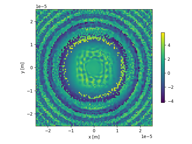
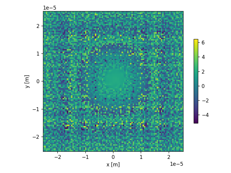
[86]:
x = solution.x
xar = np.reshape(x, (x_pixel, y_pixel))

#just for plotting the phase with dimensions
aperture.aperture = xar
moe.plotting.plot_aperture(aperture)
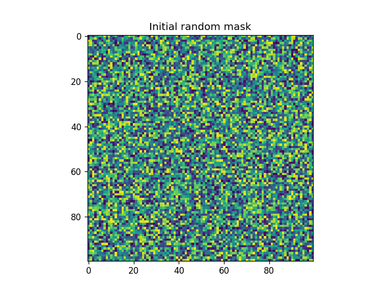
[87]:
fig = plt.figure()
xar2 = np.reshape(x0_flatten, (x_pixel, y_pixel))
plt.imshow(xar2)
plt.title("Initial random mask")
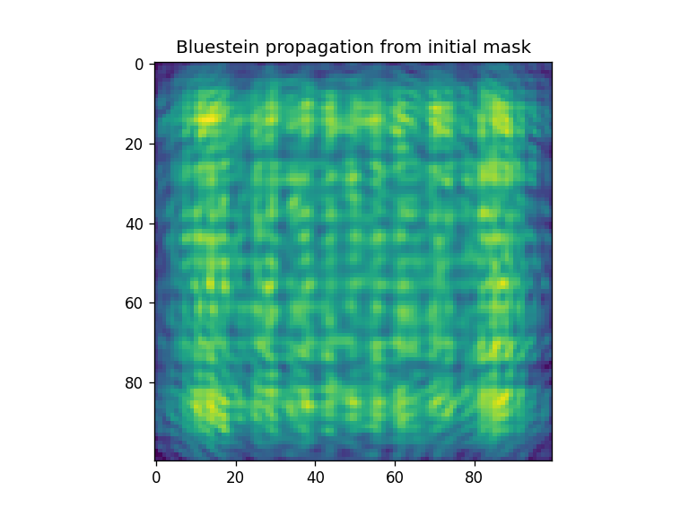
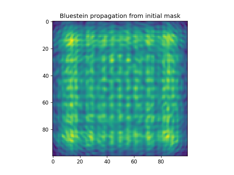
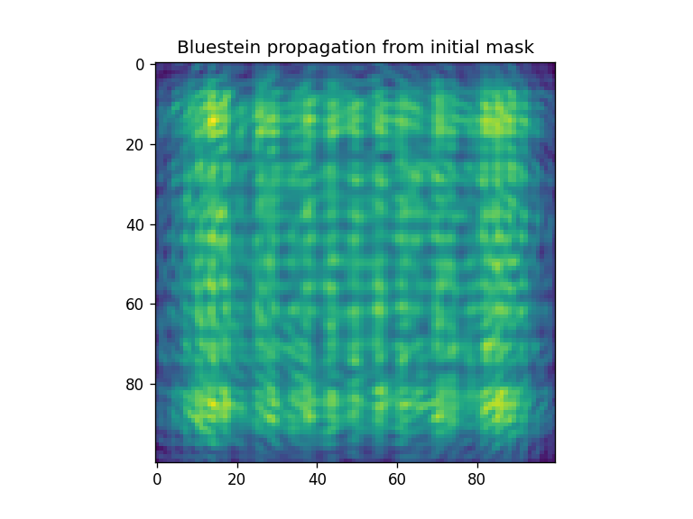
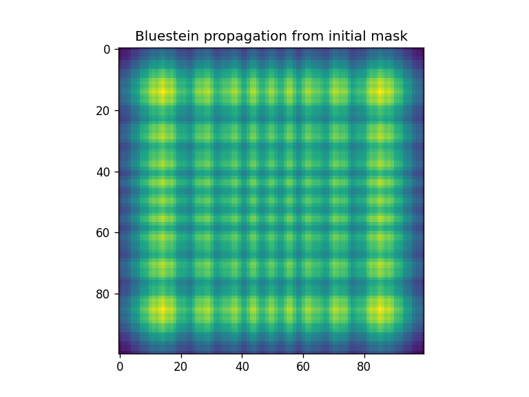
fig = plt.figure()
plt.imshow(np.abs(moe.optimizer.propagate(xar2, aperture, screen, wavelength) ) )
plt.title("Bluestein propagation from initial mask")
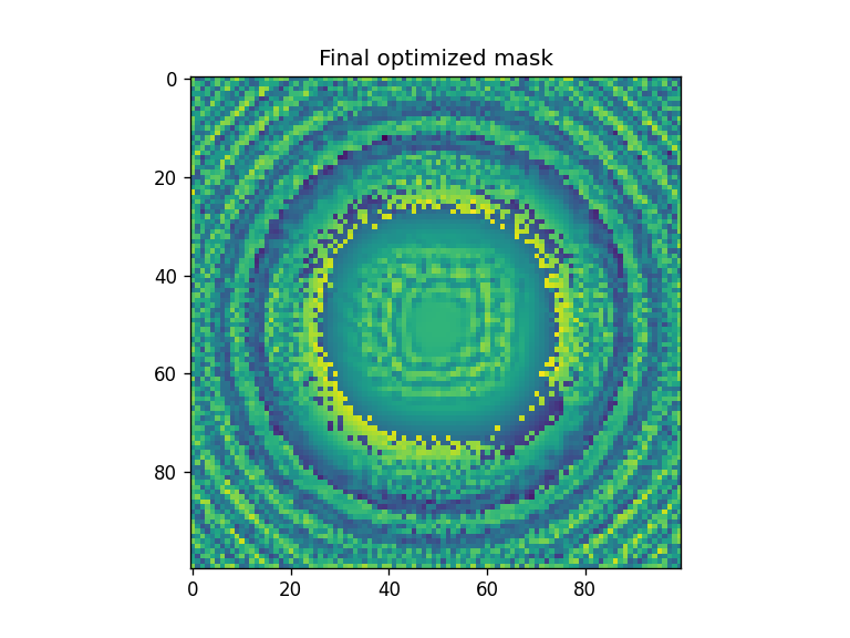
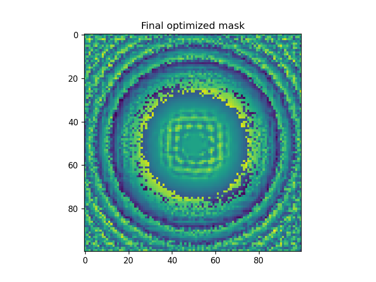
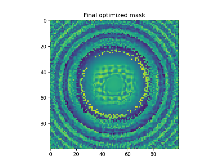
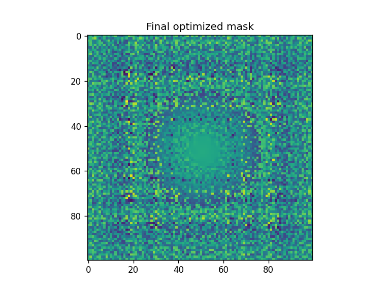
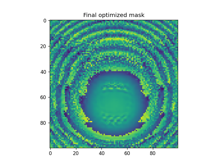
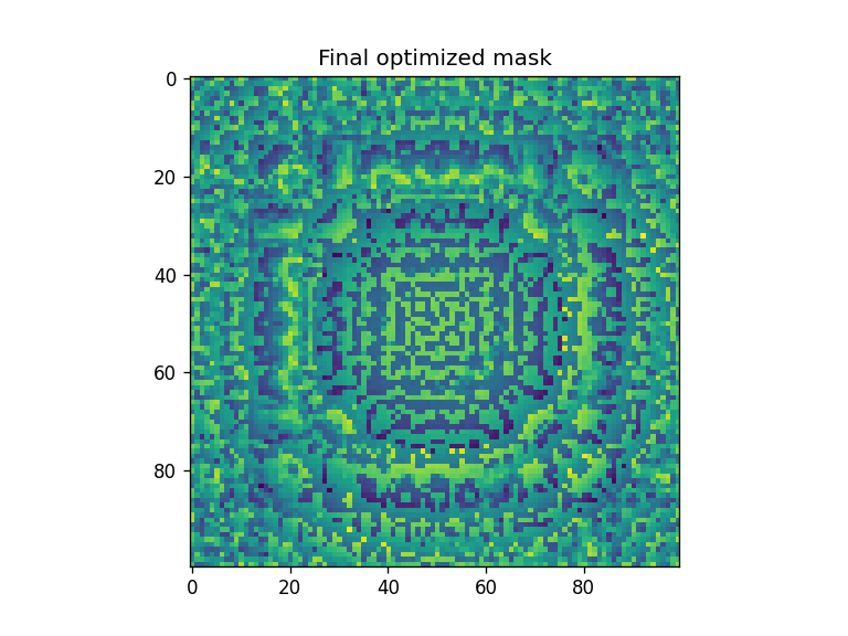
fig = plt.figure()
xar3 = np.reshape(x, (x_pixel, y_pixel))
plt.imshow(xar3)
plt.title("Final optimized mask")
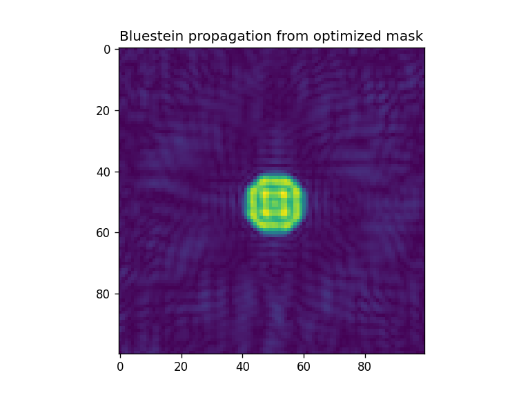
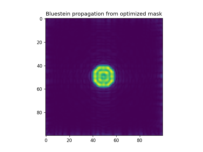
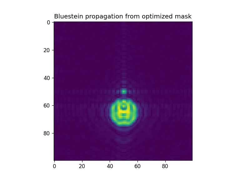
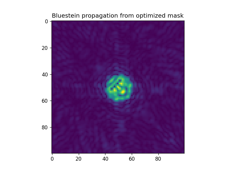
fig = plt.figure()
plt.imshow(np.abs(moe.optimizer.propagate(xar3, aperture, screen, wavelength) ) )
plt.title("Bluestein propagation from optimized mask")
fig = plt.figure()
plt.imshow(np.reshape(target, (x_pixel, y_pixel)) )
plt.title("Target")
Elapsed: 0:00:00.015431
Elapsed: 0:00:00.014934
[87]:
Text(0.5, 1.0, 'Target')


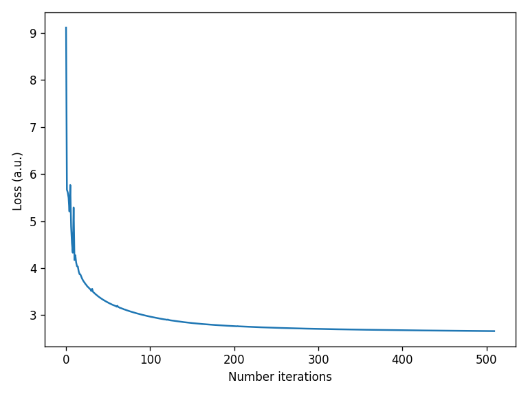
[88]:
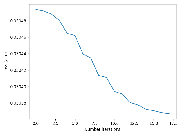
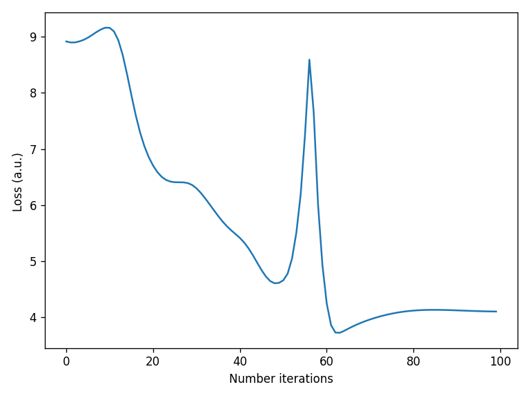
loss_vector = solution.loss_history

plt.figure()
plt.plot(loss_vector)
plt.xlabel("Number iterations")
plt.ylabel("Loss (a.u.) ")
plt.tight_layout()

Optimization with logging
The optimizer module provides an embedded logger to allow to track the optimization loss and store the parameters at each iteration step.
[89]:
# x0_flatten is your initial guess vector
logger, logfile_txt, logfile_bin, batch_list, iter_counter, batch_size, fh = moe.optimizer.setup_optimizer_logger_batch( x_size=len(x0_flatten), \
                                                                                                       batch_size=1, log_dir="logs", name="test")
[90]:
#optimize using the optimizer module  and Bluestein propagation (default)
# the initial guess is the randomly initialized x0
solution = moe.optimizer.optimize(mseloss, x0_flatten, args1=[aperture, screen, wavelength, target], verbose = 1, ftol=1e-4, logger=logger, \
                                  logfile_bin=logfile_bin, batch_list=batch_list, batch_size=batch_size, iter_counter=iter_counter, fh=fh)
Elapsed: 0:00:00.016428
Elapsed: 0:00:00.014936
Elapsed: 0:00:00.040821
Elapsed: 0:00:00.014933
Elapsed: 0:00:00.014436
Elapsed: 0:00:00.040820
Elapsed: 0:00:00.016421
Elapsed: 0:00:00.014437
Elapsed: 0:00:00.041815
Elapsed: 0:00:00.014438
Elapsed: 0:00:00.014436
Elapsed: 0:00:00.040323
Elapsed: 0:00:00.014935
Elapsed: 0:00:00.014934
Elapsed: 0:00:00.039326
Elapsed: 0:00:00.014437
Elapsed: 0:00:00.013939
Elapsed: 0:00:00.038830
Elapsed: 0:00:00.018419
Elapsed: 0:00:00.014437
Elapsed: 0:00:00.039325
Elapsed: 0:00:00.014437
Elapsed: 0:00:00.014437
Elapsed: 0:00:00.039327
Elapsed: 0:00:00.014437
Elapsed: 0:00:00.014437
Elapsed: 0:00:00.038829
Elapsed: 0:00:00.014437
Elapsed: 0:00:00.014435
Elapsed: 0:00:00.038829
Elapsed: 0:00:00.014436
Elapsed: 0:00:00.013939
Elapsed: 0:00:00.039328
Elapsed: 0:00:00.013939
Elapsed: 0:00:00.013939
Elapsed: 0:00:00.038830
Elapsed: 0:00:00.018916
Elapsed: 0:00:00.013939
Elapsed: 0:00:00.038830
Elapsed: 0:00:00.014436
Elapsed: 0:00:00.014935
Elapsed: 0:00:00.046296
Elapsed: 0:00:00.014436
Elapsed: 0:00:00.018917
Elapsed: 0:00:00.041320
Elapsed: 0:00:00.015432
Elapsed: 0:00:00.014431
Elapsed: 0:00:00.039825
Elapsed: 0:00:00.015930
Elapsed: 0:00:00.018420
Elapsed: 0:00:00.061232
Elapsed: 0:00:00.014436
Elapsed: 0:00:00.017921
Elapsed: 0:00:00.059239
`ftol` termination condition is satisfied.
Function evaluations 18, initial cost 4.6493e-04, final cost 4.6108e-04, first-order optimality 6.27e-09.
[91]:
x = solution.x
xar = np.reshape(x, (x_pixel, y_pixel))

fig = plt.figure()
xar2 = np.reshape(x0_flatten, (x_pixel, y_pixel))
plt.imshow(xar2)
plt.title("Initial random mask")

fig = plt.figure()
plt.imshow(np.abs(moe.optimizer.propagate(xar2, aperture, screen, wavelength) ) )
plt.title("Bluestein propagation from initial mask")


fig = plt.figure()
xar3 = np.reshape(x, (x_pixel, y_pixel))
plt.imshow(xar3)
plt.title("Final optimized mask")

fig = plt.figure()
plt.imshow(np.abs(moe.optimizer.propagate(xar3, aperture, screen, wavelength) ) )
plt.title("Bluestein propagation from optimized mask")

fig = plt.figure()
plt.imshow(np.reshape(target, (x_pixel, y_pixel)) )
plt.title("Target")
Elapsed: 0:00:00.026882
Elapsed: 0:00:00.018918
[91]:
Text(0.5, 1.0, 'Target')


[92]:
loss_vector = solution.loss_history

plt.figure()
plt.plot(loss_vector)
plt.xlabel("Number iterations")
plt.ylabel("Loss (a.u.) ")
plt.tight_layout()
Optimization with different forward propagators
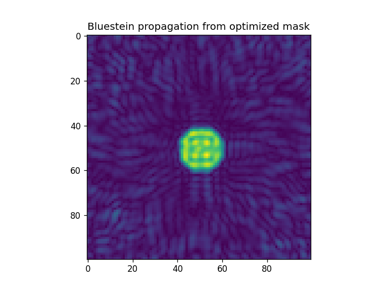
Below we demonstrate several optimizations using Bluestein, ASM and SASM propagators in the forward step. All of them yield acceptable inverse designed masks.
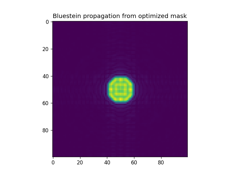
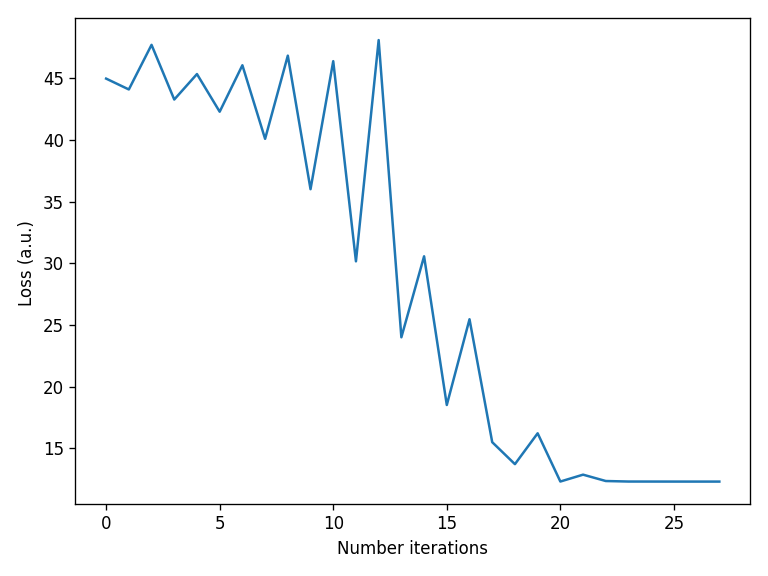
Bluestein (default)
[93]:
#optimize using the optimizer module and Bluestein propagation (default)
# the initial guess is the randomly initialized x0
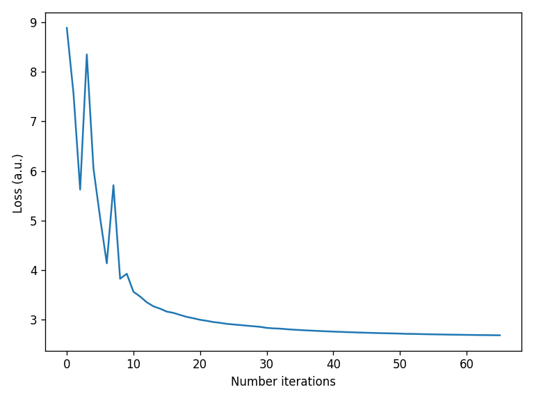
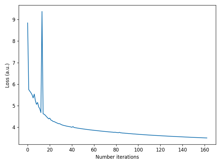
solution = moe.optimizer.optimize(logloss, x0_flatten, args1=[aperture, screen, wavelength, target, "bluestein", False], verbose = 1, ftol=1e-4)
`ftol` termination condition is satisfied.
Function evaluations 697, initial cost 4.0572e+01, final cost 3.6896e+00, first-order optimality 9.81e-04.
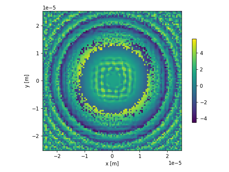
[94]:
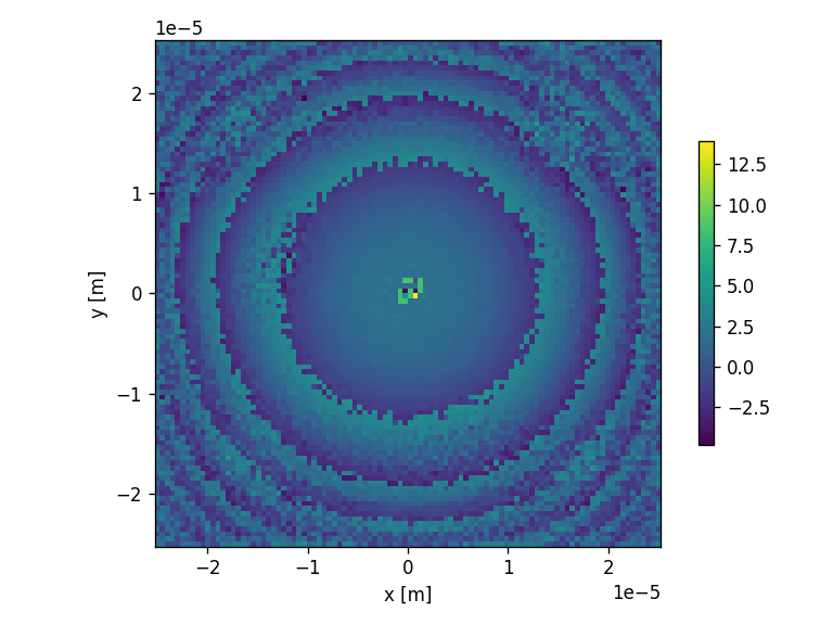
x = solution.x
xar = np.reshape(x, (x_pixel, y_pixel))

#just for plotting the phase with dimensions
aperture.aperture = xar
moe.plotting.plot_aperture(aperture)
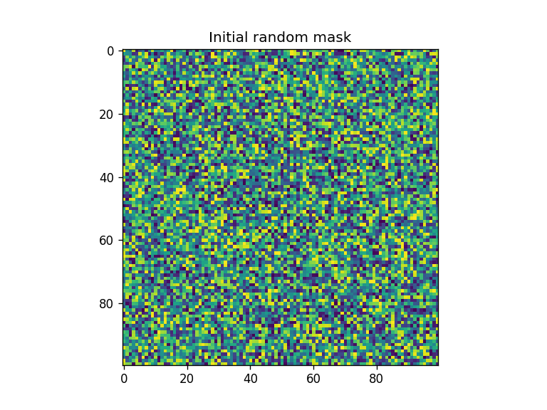
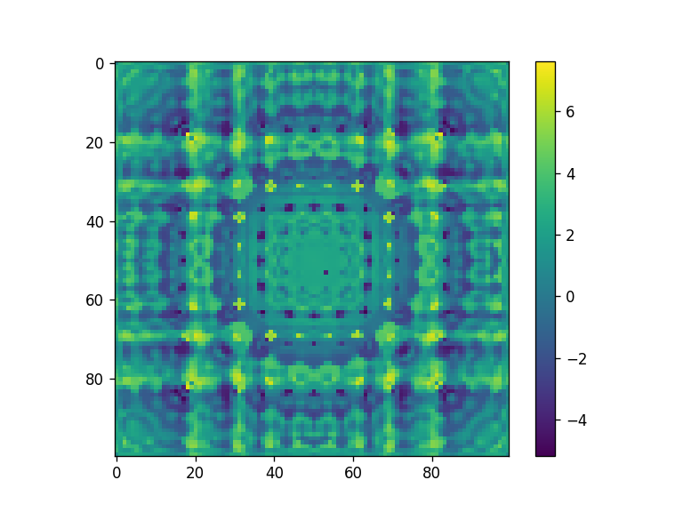
[95]:
fig = plt.figure()
xar2 = np.reshape(x0_flatten, (x_pixel, y_pixel))
plt.imshow(xar2)
plt.title("Initial random mask")
fig = plt.figure()
plt.imshow(np.abs(moe.optimizer.propagate(xar2, aperture, screen, wavelength) ) )
plt.title("Bluestein propagation from initial mask")
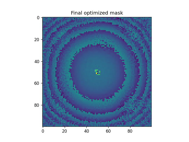
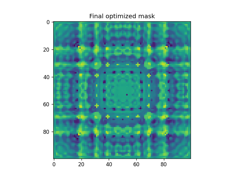
fig = plt.figure()
xar3 = np.reshape(x, (x_pixel, y_pixel))
plt.imshow(xar3)
plt.title("Final optimized mask")
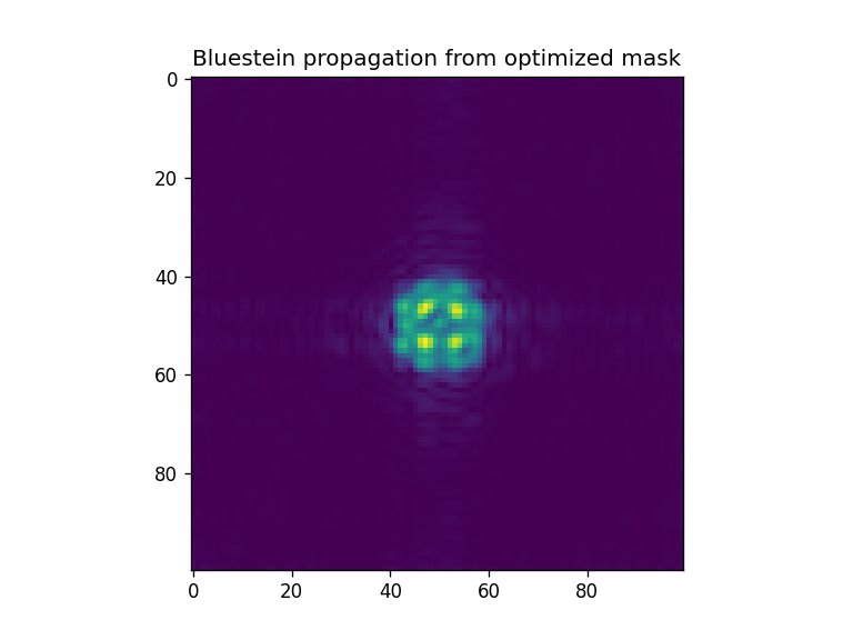
fig = plt.figure()
plt.imshow(np.abs(moe.optimizer.propagate(xar3, aperture, screen, wavelength) ) )
plt.title("Bluestein propagation from optimized mask")
fig = plt.figure()
plt.imshow(np.reshape(target, (x_pixel, y_pixel)) )
plt.title("Target")
Elapsed: 0:00:00.016428
Elapsed: 0:00:00.014935
[95]:
Text(0.5, 1.0, 'Target')


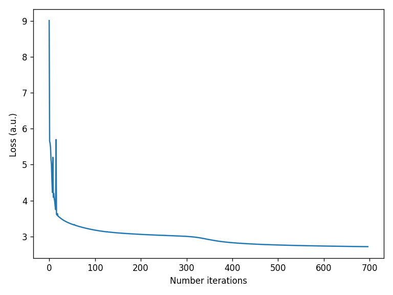
[96]:
loss_vector = solution.loss_history

plt.figure()
plt.plot(loss_vector)
plt.xlabel("Number iterations")
plt.ylabel("Loss (a.u.) ")
plt.tight_layout()
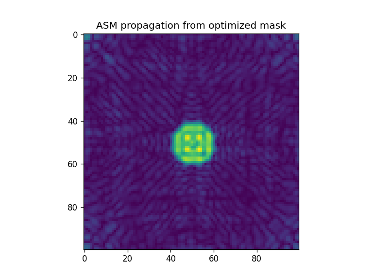
ASM
[97]:
#optimize using the optimizer module  and Bluestein propagation (default)
# the initial guess is the randomly initialized x0
solution = moe.optimizer.optimize(logloss, x0_flatten, args1=[aperture, screen, wavelength, target, "ASM", False], verbose = 1, ftol=1e-4,)
`ftol` termination condition is satisfied.
Function evaluations 510, initial cost 4.1513e+01, final cost 3.5448e+00, first-order optimality 1.45e-03.
[98]:
x = solution.x
xar = np.reshape(x, (x_pixel, y_pixel))

#just for plotting the phase with dimensions
aperture.aperture = xar
moe.plotting.plot_aperture(aperture)
[99]:
fig = plt.figure()
xar2 = np.reshape(x0_flatten, (x_pixel, y_pixel))
plt.imshow(xar2)
plt.title("Initial random mask")

fig = plt.figure()
plt.imshow(np.abs(moe.optimizer.propagate(xar2, aperture, screen, wavelength) ) )
plt.title("Bluestein propagation from initial mask")


fig = plt.figure()
xar3 = np.reshape(x, (x_pixel, y_pixel))
plt.imshow(xar3)
plt.title("Final optimized mask")

fig = plt.figure()
plt.imshow(np.abs(moe.optimizer.propagate(xar3, aperture, screen, wavelength) ) )
plt.title("Bluestein propagation from optimized mask")

fig = plt.figure()
plt.imshow(np.reshape(target, (x_pixel, y_pixel)) )
plt.title("Target")
Elapsed: 0:00:00.024393
Elapsed: 0:00:00.015432
[99]:
Text(0.5, 1.0, 'Target')


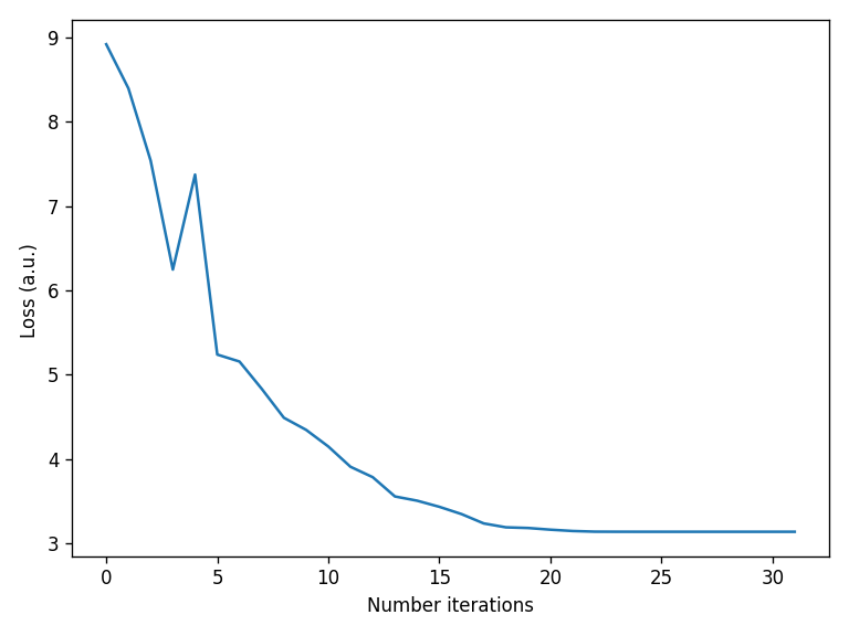
[100]:
loss_vector = solution.loss_history

plt.figure()
plt.plot(loss_vector)
plt.xlabel("Number iterations")
plt.ylabel("Loss (a.u.) ")
plt.tight_layout()
SASM
[101]:
#optimize using the optimizer module  and Bluestein propagation (default)
# the initial guess is the randomly initialized x0
solution = moe.optimizer.optimize(logloss, x0_flatten, args1=[aperture, screen, wavelength, target, "SASM", False], verbose = 1, ftol=1e-4,)
`ftol` termination condition is satisfied.
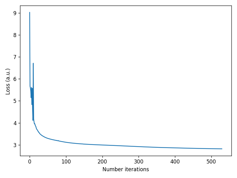
Function evaluations 530, initial cost 4.0713e+01, final cost 3.9720e+00, first-order optimality 9.30e-04.
[102]:
x = solution.x
xar = np.reshape(x, (x_pixel, y_pixel))

#just for plotting the phase with dimensions
aperture.aperture = xar
moe.plotting.plot_aperture(aperture)
[103]:
fig = plt.figure()
xar2 = np.reshape(x0_flatten, (x_pixel, y_pixel))
plt.imshow(xar2)
plt.title("Initial random mask")

fig = plt.figure()
plt.imshow(np.abs(moe.optimizer.propagate(xar2, aperture, screen, wavelength) ) )
plt.title("Bluestein propagation from initial mask")


fig = plt.figure()
xar3 = np.reshape(x, (x_pixel, y_pixel))
plt.imshow(xar3)
plt.title("Final optimized mask")

fig = plt.figure()
plt.imshow(np.abs(moe.optimizer.propagate(xar3, aperture, screen, wavelength) ) )
plt.title("Bluestein propagation from optimized mask")

fig = plt.figure()
plt.imshow(np.reshape(target, (x_pixel, y_pixel)) )
plt.title("Target")
Elapsed: 0:00:00.017424
Elapsed: 0:00:00.015930
[103]:
Text(0.5, 1.0, 'Target')


[104]:
loss_vector = solution.loss_history

plt.figure()
plt.plot(loss_vector)
plt.xlabel("Number iterations")
plt.ylabel("Loss (a.u.) ")
plt.tight_layout()
Loss function engineering
We can alter the loss function for whatever suits us best
[107]:
def logloss2(x, mask, screen, wavelength, target, propag, use_timer):
    import jax.numpy as jnp

    prop_x =  jnp.abs(moe.optimizer.propagate(np.reshape(x, (len(screen.x), len(screen.y))), mask, screen, wavelength, propagation_method=propag , use_timer=use_timer))

    diff = jnp.abs(prop_x/prop_x[int(len(screen.x)/2), int(len(screen.y)/2)] - target/jnp.max(target))**2

    res = jnp.log(jnp.sum(diff))

    return res
[108]:
## Optimization with ASM
x0 = np.random.rand(x_pixel, y_pixel)
x0_flatten = x0.flatten()

x = np.linspace(xmin, xmax, x_pixel)
y = np.linspace(ymin, ymax, y_pixel)
z = np.array([zdist])

screen = moe.Screen(x,y,z)

aperture = moe.generate.create_empty_aperture(-aperture_width/2, aperture_width/2, x_pixel, -aperture_height/2, aperture_height/2, y_pixel)

solution = moe.optimizer.optimize(logloss2, x0_flatten, args1=[aperture, screen, wavelength, target, "ASM", False], verbose = 1, ftol=1e-3,)
`ftol` termination condition is satisfied.
Function evaluations 66, initial cost 3.9460e+01, final cost 3.6099e+00, first-order optimality 5.52e-03.
[109]:
x = solution.x
xar = np.reshape(x, (x_pixel, y_pixel))

#just for plotting the phase with dimensions
aperture.aperture = xar
moe.plotting.plot_aperture(aperture)
[110]:
fig = plt.figure()
xar2 = np.reshape(x0_flatten, (x_pixel, y_pixel))
plt.imshow(xar2)
plt.title("Initial random mask")

fig = plt.figure()
plt.imshow(np.abs(moe.optimizer.propagate(xar2, aperture, screen, wavelength) ) )
plt.title("Bluestein propagation from initial mask")


fig = plt.figure()
xar3 = np.reshape(x, (x_pixel, y_pixel))
plt.imshow(xar3)
plt.title("Final optimized mask")

fig = plt.figure()
plt.imshow(np.abs(moe.optimizer.propagate(xar3, aperture, screen, wavelength) ) )
plt.title("Bluestein propagation from optimized mask")

fig = plt.figure()
plt.imshow(np.reshape(target, (x_pixel, y_pixel)) )
plt.title("Target")
Elapsed: 0:00:00.016926
Elapsed: 0:00:00.015432
[110]:
Text(0.5, 1.0, 'Target')

[111]:
loss_vector = solution.loss_history

plt.figure()
plt.plot(loss_vector)
plt.xlabel("Number iterations")
plt.ylabel("Loss (a.u.) ")
plt.tight_layout()
Target re-definition
We can alter the target for what we desire. The target can be generated from analytical or theoretical models, e.g. it could be generated as Airy pattern or Gaussian-Laguerre beam profile.
[112]:
# re-define  target

#target with offset circle
xi = np.arange(x_pixel)
yi = np.arange(y_pixel*2)
XX, YY = np.meshgrid(xi,yi)

target = np.zeros((x_pixel, y_pixel))
target[np.where(((XX-x_pixel/2- 0)**2 + (YY-y_pixel/2-15)**2) < 10**2)] = 1


fig = plt.figure()
plt.imshow(target)
[112]:
<matplotlib.image.AxesImage at 0x1838f6b8d90>
[113]:
## Optimization with ASM
x0 = np.random.rand(x_pixel, y_pixel)
x0_flatten = x0.flatten()

x = np.linspace(xmin, xmax, x_pixel)
y = np.linspace(ymin, ymax, y_pixel)
z = np.array([zdist])

screen = moe.Screen(x,y,z)

aperture = moe.generate.create_empty_aperture(-aperture_width/2, aperture_width/2, x_pixel, -aperture_height/2, aperture_height/2, y_pixel)
[114]:
solution = moe.optimizer.optimize(logloss2, x0_flatten, args1=[aperture, screen, wavelength, target, "bluestein", False], verbose = 1, ftol=1e-3,)

x = solution.x
`ftol` termination condition is satisfied.
Function evaluations 163, initial cost 3.9079e+01, final cost 6.1378e+00, first-order optimality 3.10e-03.
[115]:
x = solution.x
xar = np.reshape(x, (x_pixel, y_pixel))
[116]:
fig = plt.figure()
xar2 = np.reshape(x0_flatten, (x_pixel, y_pixel))
plt.imshow(xar2)
plt.title("Initial random mask")

fig = plt.figure()
plt.imshow(np.abs(moe.optimizer.propagate(xar2, aperture, screen, wavelength) ) )
plt.title("Bluestein propagation from initial mask")


fig = plt.figure()
xar3 = np.reshape(x, (x_pixel, y_pixel))
plt.imshow(xar3)
plt.title("Final optimized mask")

fig = plt.figure()
plt.imshow(np.abs(moe.optimizer.propagate(xar3, aperture, screen, wavelength) ) )
plt.title("Bluestein propagation from optimized mask")

fig = plt.figure()
plt.imshow(np.reshape(target, (x_pixel, y_pixel)) )
plt.title("Target")
Elapsed: 0:00:00.015931
Elapsed: 0:00:00.015433
[116]:
Text(0.5, 1.0, 'Target')
[117]:
loss_vector = solution.loss_history

plt.figure()
plt.plot(loss_vector)
plt.xlabel("Number iterations")
plt.ylabel("Loss (a.u.) ")
plt.tight_layout()
Other optimizer algorithms
By default the optimize function uses the ‘trf’ scipy algorithm. Here we exemplify ‘dogbox’ method as well. Other optimization algortihms can be used as well, namely all methods in scipy minimize, and ‘adam’ and ‘rmsprop’ from JAX’ optax package.
[118]:
### Testing constant value initial guess

#Initial guess
x0 = np.ones((x_pixel,y_pixel))
x0_flatten = x0.flatten()


#create target matrix (central cricular pattern)
xi = np.arange(x_pixel)
yi = np.arange(y_pixel)
XX, YY = np.meshgrid(xi,yi)

target = np.zeros((x_pixel, y_pixel))
target[np.where(((XX-x_pixel/2)**2 + (YY-y_pixel/2)**2) < 10**2)] = 1

target_flat = target.flatten()

fig = plt.figure()
plt.imshow(target)
[118]:
<matplotlib.image.AxesImage at 0x18395e9d250>
[119]:
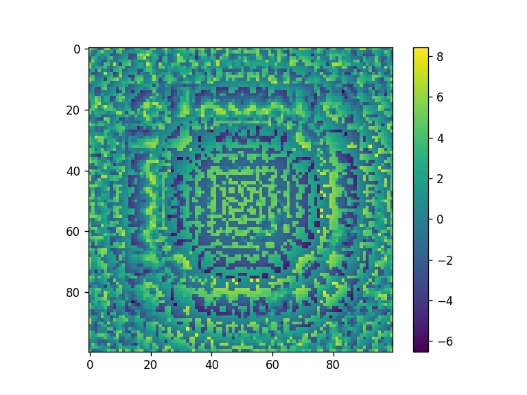
solution = moe.optimizer.optimize(logloss2, x0_flatten, args1=(aperture, screen, wavelength, target, "ASM", False), optimizer_method="dogbox", verbose=0, ftol=1e-5)

x = solution.x

fig = plt.figure()
xar = np.reshape(x, (x_pixel, y_pixel))
plt.imshow(xar)
plt.colorbar()
[119]:
<matplotlib.colorbar.Colorbar at 0x183962b9d50>
[120]:
fig = plt.figure()
xar2 = np.reshape(x0_flatten, (x_pixel, y_pixel))
plt.imshow(xar2)
plt.title("Initial mask")

fig = plt.figure()
plt.imshow(np.abs(moe.optimizer.propagate(xar2, aperture, screen, wavelength) ) )
plt.title("Bluestein propagation from initial mask")


fig = plt.figure()
xar3 = np.reshape(x, (x_pixel, y_pixel))
plt.imshow(xar3)
plt.title("Final optimized mask")

fig = plt.figure()
plt.imshow(np.abs(moe.optimizer.propagate(xar3, aperture, screen, wavelength) ) )
plt.title("Bluestein propagation from optimized mask")

fig = plt.figure()
plt.imshow(np.abs(moe.optimizer.propagate(xar3, aperture, screen, wavelength, "ASM") ) )
plt.title("ASM propagation from optimized mask")
Elapsed: 0:00:00.016926
Elapsed: 0:00:00.015432
Elapsed: 0:00:00.021406
[120]:
Text(0.5, 1.0, 'ASM propagation from optimized mask')


[121]:
loss_vector = solution.loss_history

plt.figure()
plt.plot(loss_vector)
plt.xlabel("Number iterations")
plt.ylabel("Loss (a.u.) ")
plt.tight_layout()
[122]:
#Uncomment to try any of these global optimization methods

##bounds = [(-np.pi, np.pi)]*len(x0_flatten)

#solution = moe.optimizer.optimize(logloss2, x0_flatten, args1=(aperture, screen,wavelength),  optimizer_method="dual_annealing", \
#                                  tol=1 , minimizer_kwargs={"args":(aperture, screen, wavelength), "tol": 1 },  bounds = bounds)

#solution = moe.optimizer.optimize(FOM2, x0_flatten, args1=(aperture, screen),  optimizer_method="basinhopping", tol=1 ,\
#                                  minimizer_kwargs={"args":(aperture, screen), "tol": 1 },  bounds = bounds)

#solution = moe.optimizer.optimize(FOM2, x0_flatten, args1=(aperture, screen),  optimizer_method="differential_evolution", tol=1 ,\
#                                  minimizer_kwargs={"args":(aperture, screen), "tol": 1 },  bounds = bounds)
Optimization with ‘optax’ module optimizers
[125]:
solution = moe.optimizer.optimize(logloss2, x0_flatten, args1=(aperture, screen, wavelength, target, "ASM", False), \
                                  optimizer_method="adam", verbose=0, ftol=1e-5)
[126]:
x = solution.x

fig = plt.figure()
xar = np.reshape(x, (x_pixel, y_pixel))
plt.imshow(xar)
plt.colorbar()
[126]:
<matplotlib.colorbar.Colorbar at 0x1838f5ee250>
[127]:
fig = plt.figure()
xar2 = np.reshape(x0_flatten, (x_pixel, y_pixel))
plt.imshow(xar2)
plt.title("Initial mask")

fig = plt.figure()
plt.imshow(np.abs(moe.optimizer.propagate(xar2, aperture, screen, wavelength) ) )
plt.title("Bluestein propagation from initial mask")


fig = plt.figure()
xar3 = np.reshape(x, (x_pixel, y_pixel))
plt.imshow(xar3)
plt.title("Final optimized mask")

fig = plt.figure()
plt.imshow(np.abs(moe.optimizer.propagate(xar3, aperture, screen, wavelength) ) )
plt.title("Bluestein propagation from optimized mask")

fig = plt.figure()
plt.imshow(np.abs(moe.optimizer.propagate(xar3, aperture, screen, wavelength, "ASM") ) )
plt.title("ASM propagation from optimized mask")
Elapsed: 0:00:00.015432
Elapsed: 0:00:00.016428
Elapsed: 0:00:00.015432
[127]:
Text(0.5, 1.0, 'ASM propagation from optimized mask')

[128]:
loss_vector = solution.loss_history

plt.figure()
plt.plot(loss_vector)
plt.xlabel("Number iterations")
plt.ylabel("Loss (a.u.) ")
plt.tight_layout()
Bounds during optimization
By default the optimizers are unbound. Some can be bound, such as ‘dogbox’.
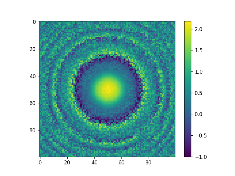
[135]:
## Optimization with bounds

solution = moe.optimizer.optimize(mseloss, x0_flatten, args1=(aperture, screen, wavelength, target, "bluestein",), optimizer_method="dogbox", \
                                  bounds =(-1, 3), ftol = 1e-12 ,xtol=1e-12, )

x = solution.x

fig = plt.figure()
xar = np.reshape(x, (x_pixel, y_pixel))
plt.imshow(xar)
plt.colorbar()
Elapsed: 0:00:00.015432
Elapsed: 0:00:00.014436
Elapsed: 0:00:00.040323
Elapsed: 0:00:00.014933
Elapsed: 0:00:00.014436
Elapsed: 0:00:00.039328
Elapsed: 0:00:00.014931
Elapsed: 0:00:00.014437
Elapsed: 0:00:00.040323
Elapsed: 0:00:00.014934
Elapsed: 0:00:00.016926
Elapsed: 0:00:00.038331
Elapsed: 0:00:00.017424
Elapsed: 0:00:00.014934
Elapsed: 0:00:00.039328
Elapsed: 0:00:00.014437
Elapsed: 0:00:00.013939
Elapsed: 0:00:00.039327
Elapsed: 0:00:00.014436
Elapsed: 0:00:00.014437
Elapsed: 0:00:00.047292
Elapsed: 0:00:00.019415
Elapsed: 0:00:00.018418
Elapsed: 0:00:00.041318
Elapsed: 0:00:00.014436
Elapsed: 0:00:00.013939
Elapsed: 0:00:00.466954
Elapsed: 0:00:00.016924
Elapsed: 0:00:00.018918
Elapsed: 0:00:00.039327
Elapsed: 0:00:00.014935
Elapsed: 0:00:00.014436
Elapsed: 0:00:00.041318
Elapsed: 0:00:00.014436
Elapsed: 0:00:00.014437
Elapsed: 0:00:00.044305
Elapsed: 0:00:00.014914
Elapsed: 0:00:00.017423
Elapsed: 0:00:00.053786
Elapsed: 0:00:00.014934
Elapsed: 0:00:00.014935
Elapsed: 0:00:00.039327
Elapsed: 0:00:00.015930
Elapsed: 0:00:00.015432
Elapsed: 0:00:00.041817
Elapsed: 0:00:00.014934
Elapsed: 0:00:00.014437
Elapsed: 0:00:00.039327
Elapsed: 0:00:00.017424
Elapsed: 0:00:00.014935
Elapsed: 0:00:00.039824
Elapsed: 0:00:00.016926
Elapsed: 0:00:00.015432
Elapsed: 0:00:00.039825
Elapsed: 0:00:00.015433
Elapsed: 0:00:00.014437
Elapsed: 0:00:00.040324
Elapsed: 0:00:00.014437
Elapsed: 0:00:00.014436
Elapsed: 0:00:00.042314
Elapsed: 0:00:00.014935
Elapsed: 0:00:00.018419
Elapsed: 0:00:00.040323
Elapsed: 0:00:00.014436
Elapsed: 0:00:00.014436
Elapsed: 0:00:00.039328
Elapsed: 0:00:00.018916
Elapsed: 0:00:00.014437
Elapsed: 0:00:00.042314
Elapsed: 0:00:00.014935
Elapsed: 0:00:00.014437
Elapsed: 0:00:00.040323
Elapsed: 0:00:00.015433
Elapsed: 0:00:00.014437
Elapsed: 0:00:00.043310
Elapsed: 0:00:00.014935
Elapsed: 0:00:00.014437
Elapsed: 0:00:00.013939
Elapsed: 0:00:00.014436
Elapsed: 0:00:00.014935
Elapsed: 0:00:00.017423
Elapsed: 0:00:00.014935
Elapsed: 0:00:00.014437
Elapsed: 0:00:00.014935
Elapsed: 0:00:00.013939
Elapsed: 0:00:00.014437
Elapsed: 0:00:00.013940
Elapsed: 0:00:00.013940
Elapsed: 0:00:00.014436
Elapsed: 0:00:00.014437
Elapsed: 0:00:00.015930
Elapsed: 0:00:00.015432
Elapsed: 0:00:00.014932
Elapsed: 0:00:00.014931
Elapsed: 0:00:00.014935
Elapsed: 0:00:00.018420
Elapsed: 0:00:00.024392
Elapsed: 0:00:00.026386
Elapsed: 0:00:00.015432
Elapsed: 0:00:00.015434
Elapsed: 0:00:00.014934
Elapsed: 0:00:00.017922
Elapsed: 0:00:00.021903
Elapsed: 0:00:00.014437
Elapsed: 0:00:00.014437
`xtol` termination condition is satisfied.
Function evaluations 40, initial cost 4.6493e-04, final cost 4.6467e-04, first-order optimality 2.12e-10.
[135]:
<matplotlib.colorbar.Colorbar at 0x183a034c1d0>
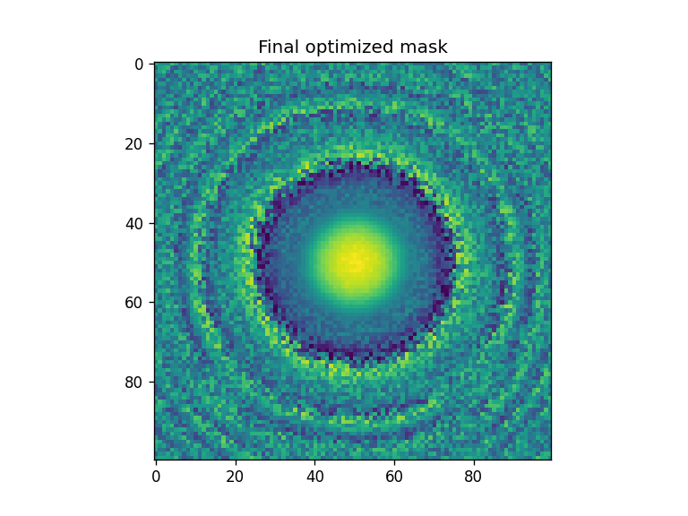
[136]:
fig = plt.figure()
xar3 = np.reshape(x, (x_pixel, y_pixel))
plt.imshow(xar3)
plt.title("Final optimized mask")
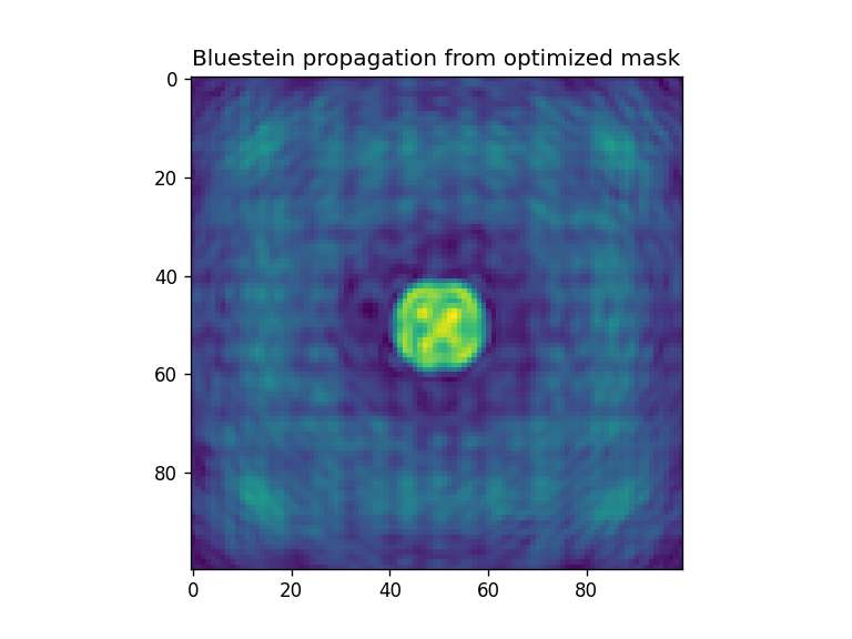
fig = plt.figure()
plt.imshow(np.abs(moe.optimizer.propagate(xar3, aperture, screen, wavelength) ) )
plt.title("Bluestein propagation from optimized mask")
Elapsed: 0:00:00.027382
[136]:
Text(0.5, 1.0, 'Bluestein propagation from optimized mask')
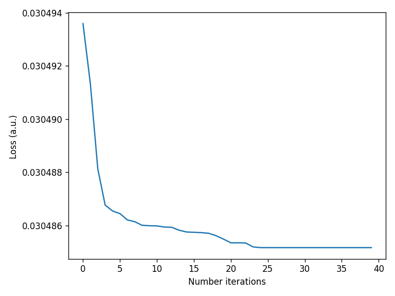
[137]:
loss_vector = solution.loss_history

plt.figure()
plt.plot(loss_vector)
plt.xlabel("Number iterations")
plt.ylabel("Loss (a.u.) ")
plt.tight_layout()
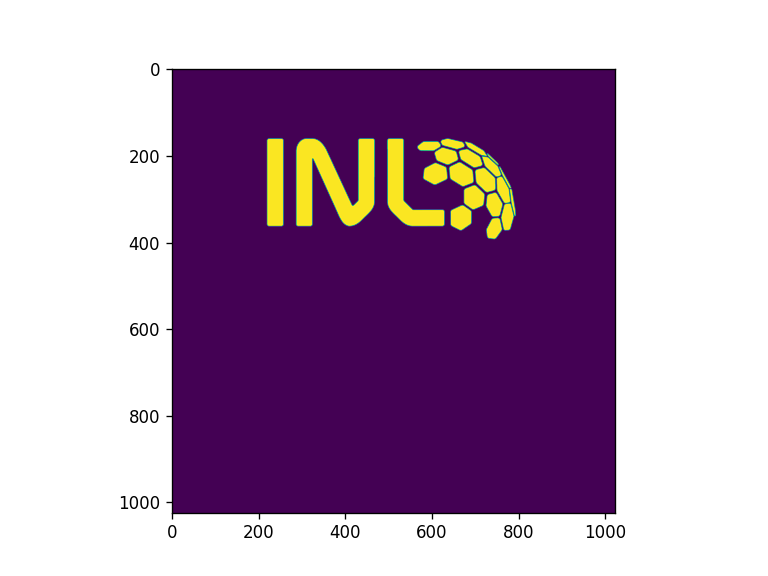
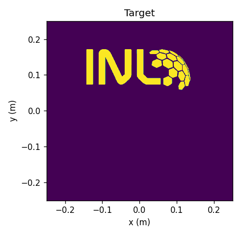
Hologram creation via inverse design
[175]:
file = "../5 - Holograms/target.png"
targetread = plt.imread(file)

x_pixel, y_pixel = np.shape(targetread)

xi = np.arange(x_pixel)
yi = np.arange(y_pixel)
XX, YY = np.meshgrid(xi,yi, indexing = 'ij')


fig = plt.figure()
plt.imshow(targetread)

targetread.shape
[175]:
(1024, 1024)
[176]:
fig = plt.figure()
plt.pcolormesh(XX,YY,targetread)
plt.gca().set_aspect('equal')
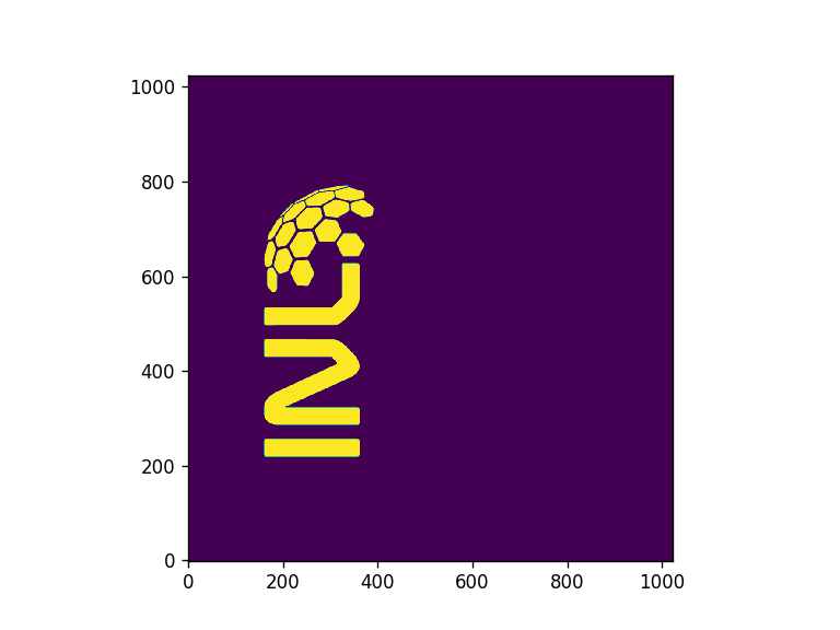
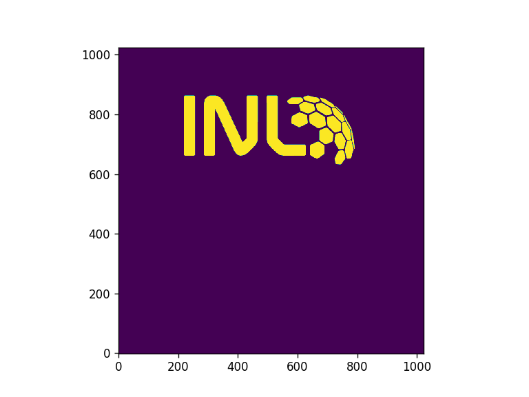
IMPORTANT the target is read as represented in the pcolormesh above in the ij indexing convention (used throughout the calculations). Hence, to have the correct representation, the axes need to be transformed.
[177]:
target = np.flip(np.rot90(targetread))

#OR THIS ONE
#targetread = np.flipud(targetread)
#targetread = np.swapaxes(targetread, 0,1)

fig = plt.figure()
plt.pcolormesh(XX,YY,target)
plt.gca().set_aspect('equal')
[178]:
#Place holders for apertures

#size of the rectangular mask
aperture_width  = 50e-6 #m
aperture_height = 50e-6

pixsize = 1e-6 #m

wavelength = 500e-9 #m
focal_length = 200e-6

zmin = wavelength
zmax = 1.2* focal_length
nzs = 500

radius = aperture_width/2

# Create Aperture
aperture1 = moe.generate.create_empty_aperture(-aperture_width/2, aperture_width/2, x_pixel, -aperture_height/2, aperture_height/2, y_pixel)
[179]:
#Define Screen

# define the wavelength used in the propagation
wavelength = 532*nano

# Define the screen size and create it

screen_width = 2.5
screen_height = 2.5
x_pixel = 1024
y_pixel = 1024


# Creates a screen in YZ plane with [-aperture_height/2, aperture_height/2] and [zmin, zmax] and
ymin, ymax = -screen_height/2, screen_height/2
xmin, xmax = -screen_width/2, screen_width/2

s = 0.2

x = np.linspace(xmin*s, xmax*s, x_pixel)
y = np.linspace(ymin*s, ymax*s, y_pixel)
z = np.array([ s ])


screen = moe.Screen(x,y,z)
[180]:
# generation of initial guesses,

#random
xrand = np.random.rand(x_pixel, y_pixel)

plt.figure()
plt.imshow(xrand)

#constant
xvalues = np.ones((x_pixel, y_pixel))

plt.figure()
plt.imshow(xvalues)
#plt.colorbar()
[180]:
<matplotlib.image.AxesImage at 0x1844a6d0b10>
[181]:
def mselossmax(x, mask, screen, wavelength, target, use_timer=True, propag="bluestein", pad=2):
    import jax.numpy as jnp

    prop_x =  jnp.abs(moe.optimizer.propagate(jnp.reshape(x, (len(screen.x), len(screen.y))), mask, screen, wavelength,\
                                             propagation_method=propag, pad_factor=pad, use_timer=use_timer))**2

    diff = jnp.abs(prop_x/jnp.max(prop_x) - target/jnp.max(target))**2

    res = jnp.sum(diff)
    return res
[182]:
solution = moe.optimizer.optimize(mselossmax, x0= xvalues.flatten(), args1=[aperture1, screen, wavelength, target, False], verbose = 1, ftol=1e-6, xtol=None,\
                                  optimizer_method='dogbox', )


x2 = solution.x
`ftol` termination condition is satisfied.
Function evaluations 88, initial cost 1.8666e+09, final cost 3.8342e+08, first-order optimality 2.55e+03.
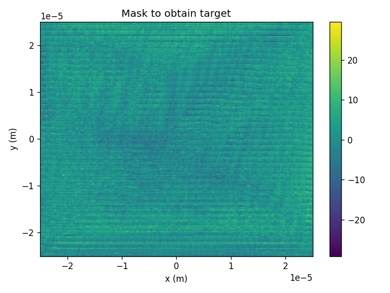
[183]:
xar3 = (np.reshape(x2, (x_pixel, y_pixel)))
# Create Aperture
aperture1 = moe.generate.create_empty_aperture(-aperture_width/2, aperture_width/2, x_pixel, -aperture_height/2, aperture_height/2, y_pixel)
fig = plt.figure()
plt.pcolormesh(aperture1.XX, aperture1.YY, xar3)
plt.title("Mask to obtain target")
plt.xlabel("x (m)")
plt.ylabel("y (m)")
plt.colorbar()
plt.tight_layout()
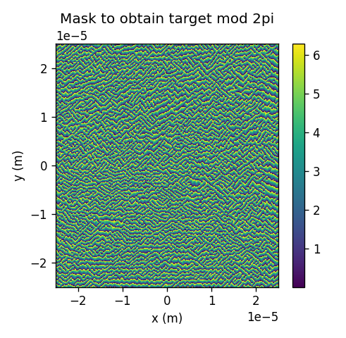
fig = plt.figure(figsize=(4.1,4))
plt.pcolormesh(aperture1.XX, aperture1.YY, (xar3)%(2*np.pi) )
plt.title("Mask to obtain target mod 2pi")
plt.xlabel("x (m)")
plt.ylabel("y (m)")
plt.colorbar()
plt.tight_layout()
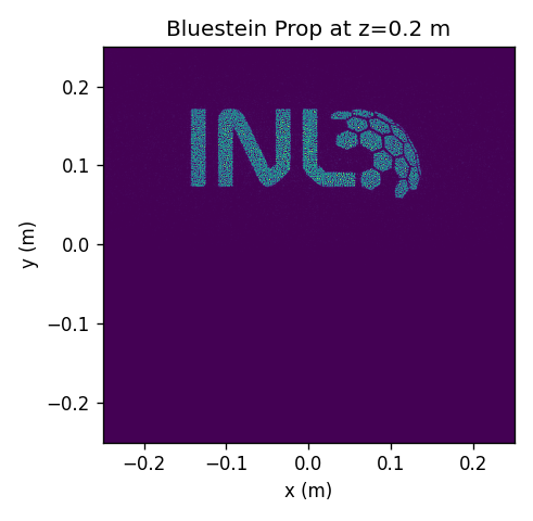
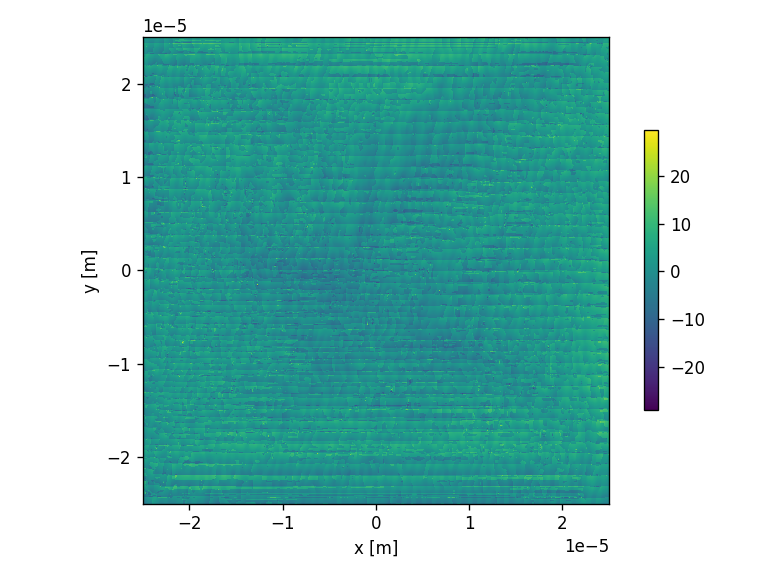
fig = plt.figure(figsize=(4.1,4))
plt.pcolormesh(screen.XX[:,:,-1], screen.YY[:,:,-1], np.abs(moe.optimizer.propagate(xar3, aperture1, screen, wavelength) )**2 )
#plt.imshow(np.abs(moe.optimizer.propagate(xar3, aperture1, screen, wavelength) )**2 )
plt.title("Bluestein Prop at z="+str(screen.z[-1])+" m")
plt.xlabel("x (m)")
plt.ylabel("y (m)")
plt.tight_layout()
fig = plt.figure(figsize=(4.1,4))
plt.pcolormesh(screen.XX[:,:,-1], screen.YY[:,:,-1], (np.reshape(target, (x_pixel, y_pixel)) ))
#plt.imshow(target)
plt.title("Target")
plt.xlabel("x (m)")
plt.ylabel("y (m)")
plt.tight_layout()
Elapsed: 0:00:00.585929
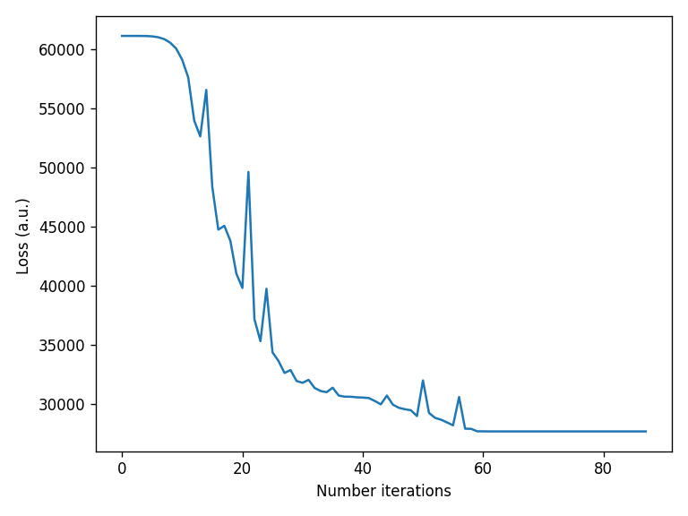
[184]:
loss_vector = solution.loss_history

plt.figure()
plt.plot(loss_vector)
plt.xlabel("Number iterations")
plt.ylabel("Loss (a.u.) ")
plt.tight_layout()
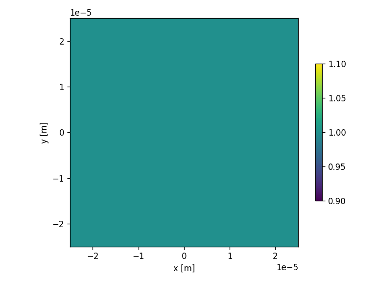
[185]:
screen = moe.Screen(x,y,z)
# Define Aperture
aperture = moe.generate.create_empty_aperture(-aperture_width/2, aperture_width/2, x_pixel, -aperture_height/2, aperture_height/2, y_pixel)
mask_amplitude = moe.generate.create_empty_aperture_from_aperture(aperture)
# Define Phase mask
mask_phase = moe.generate.create_empty_aperture_from_aperture(aperture)
mask_phase.aperture = xar3
#mask_phase.aperture = np.flipud(np.rot90(xar3)) ##use need to
mask_amplitude.aperture = mask_amplitude.aperture +1
# Plot the circular mask
moe.plotting.plot_aperture(mask_phase)
moe.plotting.plot_aperture(mask_amplitude)
# Calculates a field to use with the calculated mask
# Initialize a Field from the Aperture mask
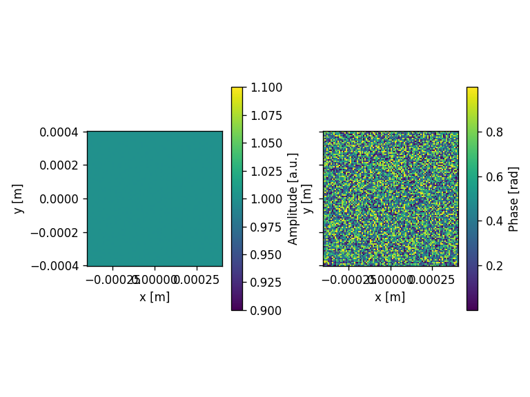
field = moe.field.create_empty_field_from_aperture(mask_phase)
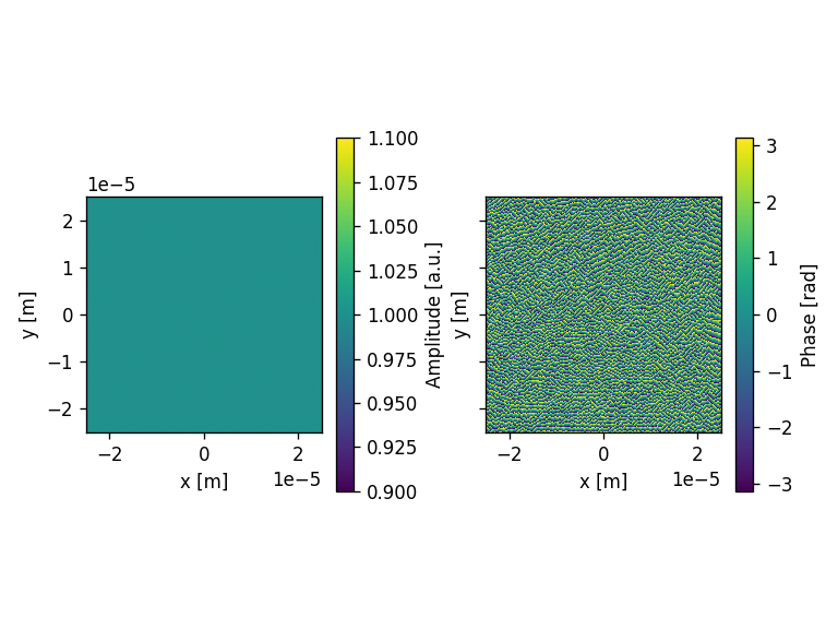
# Generate a uniform field
field = moe.field.generate_uniform_field(field, E0=1)
# Modulates the field with a given aperture that can be used either as an amplitude mask or a phase mask
field = moe.field.modulate_field(field, amplitude_mask=mask_amplitude, phase_mask=mask_phase)
# Plots the field (amplitude and phase)
moe.plotting.plot_field(field)
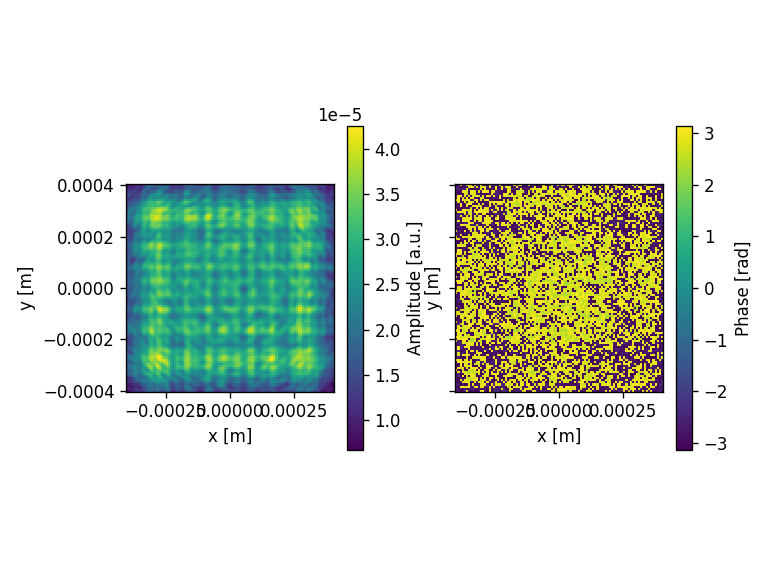
# Propagate the field with Bluestein
EXYZ = moe.propagate.Bluestein(field, screen, wavelength)
moe.plotting.plot_screen_XY(EXYZ, z=s)
Progress: [####################] 100.0%
Elapsed: 0:00:00.941867
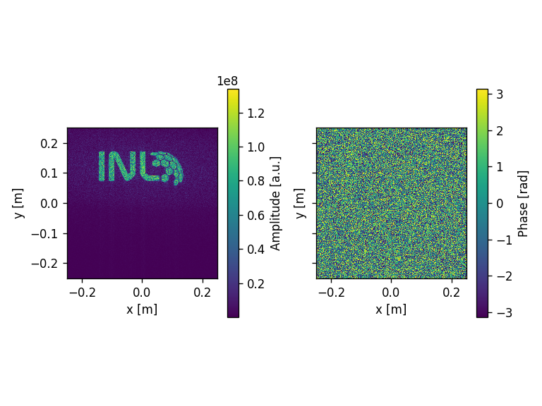
AGAIN, BEWARE all imshow will show rotated+flipped matrices, e.g. the optimization result shown below appers flipped and rotated!!!
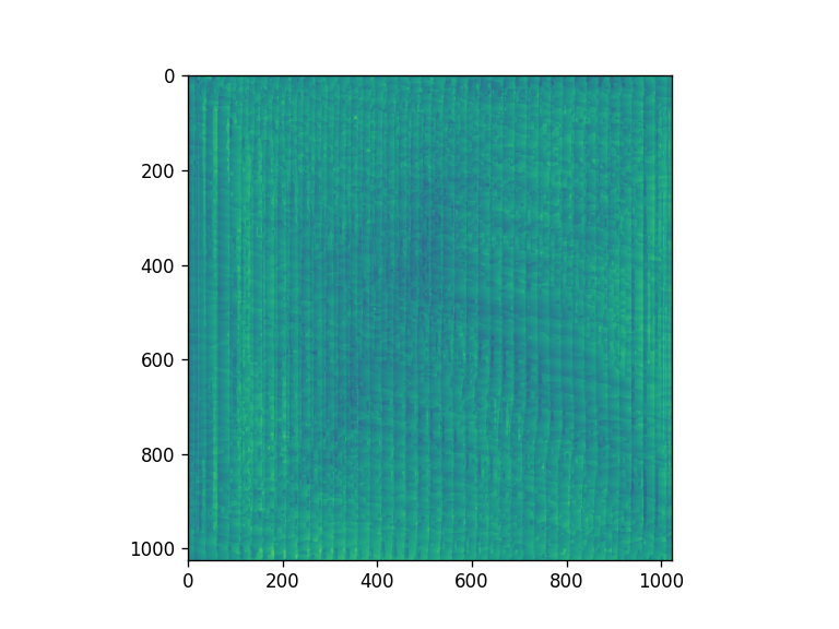
[186]:
plt.figure()
plt.imshow(xar3)
[186]:
<matplotlib.image.AxesImage at 0x183987eb510>
Optimization of ensembles of optical elements
[187]:
###Import two surfaces - doublet

#number of pixels
x_pixel = 100
y_pixel = 100

a1_phase = np.random.rand(x_pixel, y_pixel) #np.genfromtxt("asph1_phase.csv", delimiter=',')
a1_inten = a1_phase * 0 #np.genfromtxt("asph1_inten.csv", delimiter=',')

a2_phase = np.random.rand(x_pixel, y_pixel) #np.genfromtxt("asph2_phase.csv", delimiter=',')
a2_inten = a2_phase * 0 #np.genfromtxt("asph2_inten.csv", delimiter=',')


#size of the rectangular mask
aperture_width  = 800e-6 #m
aperture_height = 800e-6

pixsize = 8e-6 #m

wavelength = 550e-9

dist1 = 40e-3
dist2 = 50e-3

zmin1 = wavelength
zmax1 = dist1
nzs = 2

zmin2 = wavelength
zmax2 = dist2
nzs = 2

radius = aperture_width/2


asph1_mask_phase = moe.generate.create_empty_aperture(-aperture_width/2, aperture_width/2, x_pixel, -aperture_height/2, aperture_height/2, y_pixel)
asph1_mask_phase.aperture = a1_phase

asph1_mask_inten = moe.generate.create_empty_aperture_from_aperture(asph1_mask_phase)
asph1_mask_inten.aperture = a1_inten

asph2_mask_phase = moe.generate.create_empty_aperture(-aperture_width/2, aperture_width/2, x_pixel, -aperture_height/2, aperture_height/2, y_pixel)
asph2_mask_phase.aperture = a2_phase

asph2_mask_inten = moe.generate.create_empty_aperture_from_aperture(asph2_mask_phase)
asph2_mask_inten.aperture = a2_inten

aperture = moe.generate.create_empty_aperture_from_aperture(asph2_mask_phase)
mask = moe.generate.circular_aperture(aperture, radius=radius*10)

aperture_array_phase = [asph1_mask_phase, asph2_mask_phase]
aperture_array_amp = [mask,]*len(aperture_array_phase)

############################
## Define the screens
x1 = asph1_mask_phase.x
y1 = asph1_mask_phase.y
z1 = np.linspace(zmin1, zmax1, nzs)

screen1 = moe.field.Screen(x1,y1,z1)

x2 = asph2_mask_phase.x
y2 = asph2_mask_phase.y
z2 = np.linspace(zmin2, zmax2, nzs)

screen2 = moe.field.Screen(x2,y2,z2)


screen_array = [screen1, screen2]

##################################
#Wavelengths
wavelength_array = [wavelength]

###############################
#input field

field_input = moe.field.create_empty_field_from_aperture(aperture)
field_input = moe.field.generate_uniform_field(field_input, E0=1)
input_light_field = field_input

##create ensemble
ensemble = moe.ensemble.Ensemble(aperture_array_amp, aperture_array_phase, screen_array,  wavelength_array, input_light_field)
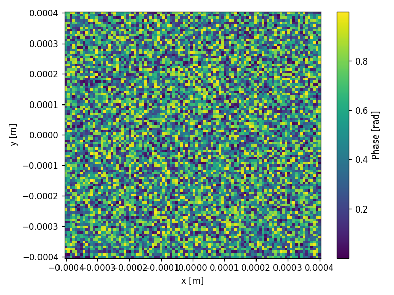
[188]:
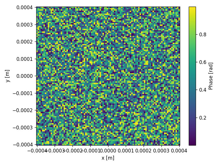
#the initial arrays are two random matrices represented below

fig = plt.figure()
plt.pcolormesh(aperture_array_phase[0].XX, aperture_array_phase[0].YY, aperture_array_phase[0].aperture)
plt.colorbar(label ="Phase [rad]")
plt.xlabel("x [m]")
plt.ylabel("y [m]")
plt.tight_layout()

fig = plt.figure()
plt.pcolormesh(aperture_array_phase[1].XX, aperture_array_phase[1].YY, aperture_array_phase[1].aperture)
plt.colorbar(label ="Phase [rad]")
plt.xlabel("x [m]")
plt.ylabel("y [m]")
plt.tight_layout()
[189]:
prop_methods = ["bluestein", "bluestein"]
EXY_array2 = [moe.propagate.propagate_through_ensemble(ensemble, wavelength, propagation_methods_array=prop_methods) for wavelength in wavelength_array]
Surface #1
Progress: [####################] 100.0%
Elapsed: 0:00:00.009459
Surface #2
Progress: [####################] 100.0%
Elapsed: 0:00:00.018420
[190]:
x0_flatten = (np.array([aperture_array_phase[0].aperture.flatten(), aperture_array_phase[1].aperture.flatten()]) ).flatten()
x0_flatten.shape, a1_phase.shape
[190]:
((20000,), (100, 100))
[191]:
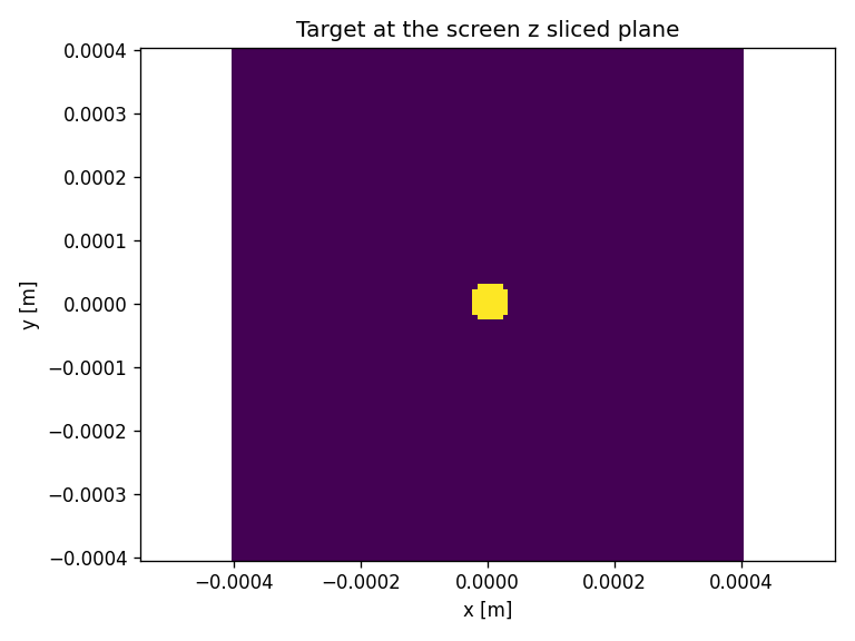
xi = np.arange(x_pixel)
yi = np.arange(y_pixel)
XX, YY = np.meshgrid(xi,yi, indexing='ij')

target = np.zeros((x_pixel, y_pixel))
target[np.where(((XX-x_pixel/2- 0)**2 + (YY-y_pixel/2-0)**2) < 4**2)] = 1

target_flat = target.flatten()

fig = plt.figure()
plt.pcolormesh(screen_array[-1].XX[:,:,-1], screen_array[-1].YY[:,:,-1], target )
plt.axis("equal")
plt.xlabel("x [m]")
plt.ylabel("y [m]")
plt.title("Target at the screen z sliced plane")
plt.tight_layout()
[192]:
def loss(x, mask, screen_array, wavelength, target, use_timer=True, propag="bluestein"):
    import jax.numpy as jnp

    #prop_x =  np.abs(moe.optimizer.propagate(np.reshape(x, (len(screen.x), len(screen.y))), mask, screen, wavelength, propagation_method=propag))
    xar1 = jnp.reshape(x[0:int(len(x)/2)], (len(screen_array[0].x), len(screen_array[0].y)))
    xar2 = jnp.reshape(x[int(len(x)/2):], (len(screen_array[0].x), len(screen_array[0].y)))
    xar=[xar1, xar2]

    prop_x = moe.optimizer.propagate(xar, aperture=aperture_array_phase, screen=screen_array , wavelength=wavelength_array, \
          mask_amp = aperture_array_amp, circ_radius=None, input_field="uniform", E0=1, \
          propagation_method=["ASM","ASM"], pad_factor=2, modedef = "czt", ensemble_mode=True , corr=1e5, use_timer=use_timer  )**2


    diff = jnp.abs(prop_x/jnp.sum(prop_x) - target/jnp.max(target))**2

    res = np.sum(diff)

    return res
[193]:
solution = moe.optimizer.optimize(loss, x0_flatten, args1=[aperture, screen_array, wavelength, target, False], verbose = 1, ftol=1e-4,)

x = solution.x
Elapsed: 0:00:00.073677
Elapsed: 0:00:00.061729
Elapsed: 0:00:00.078655
Elapsed: 0:00:00.063719
Elapsed: 0:00:00.139389
Elapsed: 0:00:00.139389
Elapsed: 0:00:00.062723
Elapsed: 0:00:00.064716
Elapsed: 0:00:00.060235
Elapsed: 0:00:00.059242
Elapsed: 0:00:00.115987
Elapsed: 0:00:00.112510
Elapsed: 0:00:00.048783
Elapsed: 0:00:00.048786
Elapsed: 0:00:00.069694
Elapsed: 0:00:00.044307
Elapsed: 0:00:00.068698
Elapsed: 0:00:00.065713
Elapsed: 0:00:00.066707
Elapsed: 0:00:00.061729
Elapsed: 0:00:00.115490
Elapsed: 0:00:00.116988
Elapsed: 0:00:00.057746
Elapsed: 0:00:00.050778
Elapsed: 0:00:00.041816
Elapsed: 0:00:00.044306
Elapsed: 0:00:00.058742
Elapsed: 0:00:00.044804
Elapsed: 0:00:00.056751
Elapsed: 0:00:00.071191
Elapsed: 0:00:00.130923
Elapsed: 0:00:00.131426
Elapsed: 0:00:00.062722
Elapsed: 0:00:00.046795
Elapsed: 0:00:00.059738
Elapsed: 0:00:00.044805
Elapsed: 0:00:00.070695
Elapsed: 0:00:00.053264
Elapsed: 0:00:00.062225
Elapsed: 0:00:00.060239
Elapsed: 0:00:00.126940
Elapsed: 0:00:00.099566
Elapsed: 0:00:00.050779
Elapsed: 0:00:00.060732
Elapsed: 0:00:00.053762
Elapsed: 0:00:00.060238
Elapsed: 0:00:00.076166
Elapsed: 0:00:00.069693
Elapsed: 0:00:00.055759
Elapsed: 0:00:00.063721
Elapsed: 0:00:00.098068
Elapsed: 0:00:00.111016
Elapsed: 0:00:00.061227
Elapsed: 0:00:00.050777
Elapsed: 0:00:00.045301
Elapsed: 0:00:00.045799
Elapsed: 0:00:00.057746
Elapsed: 0:00:00.068698
Elapsed: 0:00:00.067704
Elapsed: 0:00:00.064719
Elapsed: 0:00:00.111509
Elapsed: 0:00:00.105039
Elapsed: 0:00:00.059733
Elapsed: 0:00:00.046297
Elapsed: 0:00:00.056254
Elapsed: 0:00:00.055757
Elapsed: 0:00:00.057743
Elapsed: 0:00:00.062725
Elapsed: 0:00:00.064218
Elapsed: 0:00:00.065217
Elapsed: 0:00:00.131919
Elapsed: 0:00:00.108523
Elapsed: 0:00:00.052272
Elapsed: 0:00:00.047789
Elapsed: 0:00:00.052768
Elapsed: 0:00:00.045302
Elapsed: 0:00:00.067704
Elapsed: 0:00:00.062722
Elapsed: 0:00:00.066707
Elapsed: 0:00:00.058247
Elapsed: 0:00:00.111512
Elapsed: 0:00:00.107031
Elapsed: 0:00:00.048783
Elapsed: 0:00:00.051275
Elapsed: 0:00:00.057745
Elapsed: 0:00:00.046297
Elapsed: 0:00:00.058742
Elapsed: 0:00:00.062266
Elapsed: 0:00:00.044306
Elapsed: 0:00:00.042313
Elapsed: 0:00:00.120971
Elapsed: 0:00:00.116986
Elapsed: 0:00:00.063719
Elapsed: 0:00:00.069197
Elapsed: 0:00:00.048289
Elapsed: 0:00:00.050779
Elapsed: 0:00:00.121962
Elapsed: 0:00:00.124954
Elapsed: 0:00:00.054755
Elapsed: 0:00:00.048289
Elapsed: 0:00:00.056751
Elapsed: 0:00:00.044805
Elapsed: 0:00:00.054758
Elapsed: 0:00:00.067203
Elapsed: 0:00:00.071685
Elapsed: 0:00:00.065715
Elapsed: 0:00:00.132418
Elapsed: 0:00:00.113504
Elapsed: 0:00:00.058245
Elapsed: 0:00:00.057249
Elapsed: 0:00:00.050274
Elapsed: 0:00:00.048288
Elapsed: 0:00:00.063720
Elapsed: 0:00:00.075170
Elapsed: 0:00:00.050777
Elapsed: 0:00:00.059741
Elapsed: 0:00:00.059736
Elapsed: 0:00:00.058244
Elapsed: 0:00:00.050280
Elapsed: 0:00:00.067706
Elapsed: 0:00:00.107525
Elapsed: 0:00:00.109521
Elapsed: 0:00:00.056751
Elapsed: 0:00:00.053764
Elapsed: 0:00:00.046795
Elapsed: 0:00:00.059242
Elapsed: 0:00:00.134908
Elapsed: 0:00:00.115493
Elapsed: 0:00:00.047787
Elapsed: 0:00:00.056253
Elapsed: 0:00:00.048786
Elapsed: 0:00:00.047791
Elapsed: 0:00:00.130427
Elapsed: 0:00:00.118483
Elapsed: 0:00:00.062222
Elapsed: 0:00:00.046298
Elapsed: 0:00:00.052769
Elapsed: 0:00:00.060736
Elapsed: 0:00:00.114495
Elapsed: 0:00:00.102053
Elapsed: 0:00:00.052767
Elapsed: 0:00:00.058743
Elapsed: 0:00:00.062226
Elapsed: 0:00:00.044306
Elapsed: 0:00:00.108521
Elapsed: 0:00:00.112504
`ftol` termination condition is satisfied.
Function evaluations 28, initial cost 1.0120e+03, final cost 7.5699e+01, first-order optimality 1.37e-01.
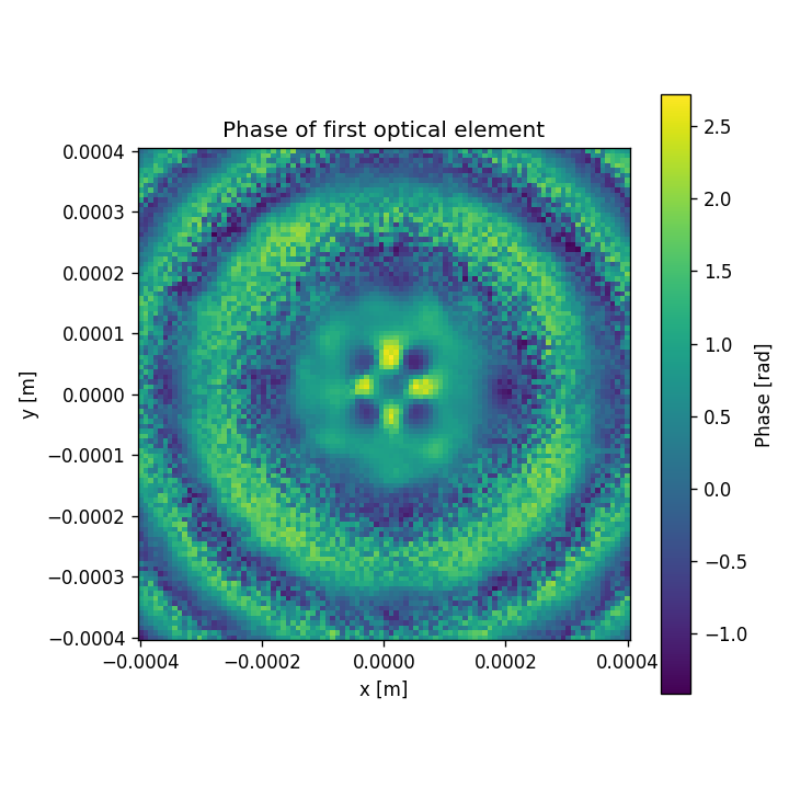
[194]:
d1 = np.reshape(x[0:int(len(x)/2)], (len(screen_array[0].x), len(screen_array[0].y)))
d2 = np.reshape(x[int(len(x)/2):], (len(screen_array[0].x), len(screen_array[0].y)))
fig = plt.figure(figsize = (6,6))
xar3 = np.reshape(d1, (x_pixel, y_pixel))
plt.pcolormesh(aperture_array_phase[0].XX, aperture_array_phase[0].YY, xar3)
plt.colorbar(label = "Phase [rad]", shrink=0.8)
plt.title("Phase of first optical element")
plt.xlabel("x [m]")
plt.ylabel("y [m]")
plt.gca().set_aspect('equal')
plt.tight_layout()
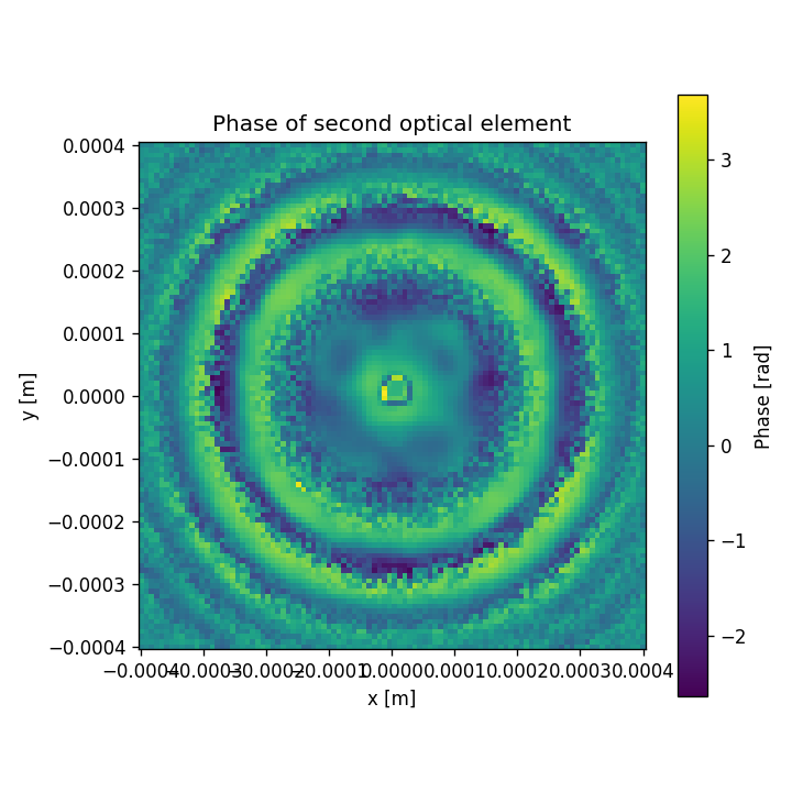
fig = plt.figure(figsize = (6,6))
xar4 = np.reshape(d2, (x_pixel, y_pixel))
plt.pcolormesh(aperture_array_phase[1].XX, aperture_array_phase[1].YY, xar4)
plt.colorbar(label = "Phase [rad]", shrink=0.8)
plt.title("Phase of second optical element")
plt.xlabel("x [m]")
plt.ylabel("y [m]")
plt.gca().set_aspect('equal')
plt.tight_layout()
Ep = moe.optimizer.propagate(xar=[d1, d2], aperture=aperture_array_phase, screen=screen_array , wavelength=wavelength_array, \
mask_amp = aperture_array_amp, circ_radius=None, input_field="uniform", E0=1, \
propagation_method=["ASM","ASM"], pad_factor=2, modedef = "czt", ensemble_mode=True )
fig = plt.figure(figsize = (6,6))
plt.pcolormesh(screen_array[-1].XX[:,:,-1], screen_array[-1].YY[:,:,-1], (np.abs(Ep) )**2)
plt.colorbar(label = "Intensity [a.u.]", shrink=0.8)
plt.title("Propagation through ensemble with ASM-CZT")
plt.xlabel("x [m]")
plt.ylabel("y [m]")
plt.gca().set_aspect('equal')
plt.tight_layout()
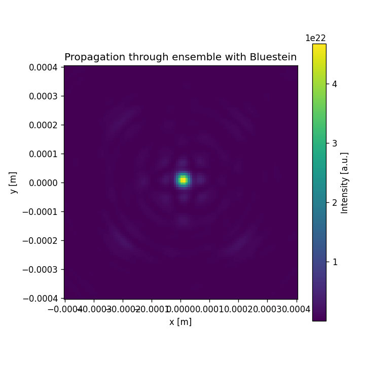
Ep = moe.optimizer.propagate(xar=[d1, d2], aperture=aperture_array_phase, screen=screen_array , wavelength=wavelength_array, \
mask_amp = aperture_array_amp, circ_radius=None, input_field="uniform", E0=1, \
propagation_method=["bluestein","bluestein"], pad_factor=2, ensemble_mode=True , corr=1e10 )
fig = plt.figure(figsize = (6,6))
plt.pcolormesh(screen_array[-1].XX[:,:,-1], screen_array[-1].YY[:,:,-1], (np.abs(Ep) )**2)
plt.colorbar(label = "Intensity [a.u.]", shrink=0.8)
plt.title("Propagation through ensemble with Bluestein")
plt.xlabel("x [m]")
plt.ylabel("y [m]")
plt.gca().set_aspect('equal')
plt.tight_layout()
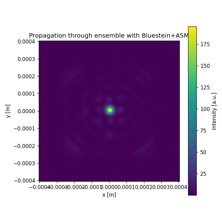
Ep = moe.optimizer.propagate(xar=[d1, d2], aperture=aperture_array_phase, screen=screen_array , wavelength=wavelength_array, \
mask_amp = aperture_array_amp, circ_radius=None, input_field="uniform", E0=1, \
propagation_method=["bluestein","ASM"], pad_factor=2, ensemble_mode=True , corr=1e10 )
fig = plt.figure(figsize = (6,6))
plt.pcolormesh(screen_array[-1].XX[:,:,-1], screen_array[-1].YY[:,:,-1], (np.abs(Ep) )**2)
plt.colorbar(label = "Intensity [a.u.]", shrink=0.8)
plt.title("Propagation through ensemble with Bluestein+ASM")
plt.xlabel("x [m]")
plt.ylabel("y [m]")
plt.gca().set_aspect('equal')
plt.tight_layout()
Elapsed: 0:00:00.062725
Elapsed: 0:00:00.058742
Elapsed: 0:00:00.029869
Elapsed: 0:00:00.030864
Elapsed: 0:00:00.030367
Elapsed: 0:00:00.060733

[195]:
loss_vector = solution.loss_history

plt.figure()
plt.plot(loss_vector)
plt.xlabel("Number iterations")
plt.ylabel("Loss (a.u.) ")
plt.tight_layout()
[ ]:
[ ]:
[ ]: